Clustering of Fortune 500 companies based on Twitter activity
1. Importing required packages
# twitter loader
import sys
sys.path.append('[...]/GetOldTweets-python/')
import got3

# misc packages
from collections import defaultdict
import pandas as pd
import numpy as np
import pickle as pkl
from math import isnan
import os
from time import time

# Packages for scraping
from fake_useragent import UserAgent
import re
import requests as req
from bs4 import BeautifulSoup
from urllib.parse import urljoin

# Packages for cleaning text
from string import digits, punctuation
from nltk.corpus import stopwords
from textwrap import wrap

# Packages for unsupervised learning
from sklearn.feature_extraction.text import  TfidfVectorizer, CountVectorizer
from sklearn.decomposition import PCA, NMF, TruncatedSVD
from sklearn.preprocessing import MinMaxScaler

# Packages for plotting
import matplotlib.pyplot as plt
%matplotlib inline
import seaborn as sns
sns.set()
2. Setup engine to scrape Twitter
To scrape Twitter and reach more-than-a-week-old tweets we need to bypass the official API. I found this neat solution online, called GetOldTweets-python.
Quoting their documentation:
> Twitter Official API has the bother limitation of time constraints, you can’t get older tweets than a week.
Some tools provide access to older tweets but in the most of them you have to spend some money before.
I was searching other tools to do this job but I didn’t found it, so after analyze how Twitter Search
through browser works I understand its flow.
Basically when you enter on Twitter page a scroll loader starts, if you scroll down you start to get more and more tweets,
all through calls to a JSON provider. After mimic we get the best advantage of Twitter Search on browsers,
it can search the deepest oldest tweets.
def recent_tweets(username=False, query=False, max_tweets=10):
    '''
    Pulling recent tweets from a Twitter username and query custom combination.

    Input: username, query (e.g. a hashtag), number of tweets to pull
    Output: List of tweet text and metadata

    '''

    d_tweets = defaultdict(list)
    tweetCriteria = got3.manager.TweetCriteria().setMaxTweets(max_tweets)

    if username and query:
        tweetCriteria = tweetCriteria.setUsername(username).setQuerySearch(query)
    elif username and query==False:
        tweetCriteria = tweetCriteria.setUsername(username)
    elif username==False and query:
        tweetCriteria = tweetCriteria.setQuerySearch(query)
    else:
        return False
    tweets = got3.manager.TweetManager.getTweets(tweetCriteria)
    for i in range(max_tweets):
        #print(f'Retrieving tweet #{i+1} of {max_tweets}')
        try:
            tweet_current = tweets[i]
            d_tweets[tweet_current.id] = [tweet_current.permalink, tweet_current.username, tweet_current.date,
                                  tweet_current.text, tweet_current.retweets, tweet_current.favorites,
                                  tweet_current.mentions, tweet_current.hashtags, tweet_current.geo]
        except:
            return False
    return d_tweets
def tweet_dict_into_df(d_tweets):
'''
Create a dataframe from pulled tweets
'''
df = pd.DataFrame.from_dict(d_tweets, orient='index', dtype=None).reset_index()
df.columns=['id','permalink','username','date','text','retweets','favorites','mentions','hashtags','geo']
return dfdef tweet_loader(current_username=False,current_query=False,current_tweets=10):
'''
A function that pulls together pulling the tweet, putting it into a dataframe then saving it one-by-one
(in case internet collapses)
'''
if current_query and current_username:
naming = current_query + '_' + current_username
elif current_query and current_username==False:
naming = current_query
elif current_query==False and current_username:
naming = current_username
print(f'Downloading {current_tweets} tweets for {naming}')
d_tweets = recent_tweets(username=current_username, query=current_query, max_tweets=current_tweets)
if d_tweets:
print(f'Saving to df')
df = tweet_dict_into_df(d_tweets)
filename = time.strftime("%Y%m%d-%H%M%S") + '_' + naming + '_recent_' + str(current_tweets) + '_tweets.pkl'
print(f'Saving dataframe as {filename}')
df.to_pickle(filename)
return df
else:
return Falsedef twitter_account_search():
'''
As a subject of this project, I decided to use a list of Fortune 500 companies for clustering.
1. I first obtained the website urls' of the companies via BeautifulSoup
2. Then I opened the website of each company and looked for twitter ids using RegEx
3. Saved each companies' Twitter ID where it was found
'''
ua = UserAgent()
header = {'User-Agent': ua.random}
url_fortune = 'https://www.zyxware.com/articles/4344/list-of-fortune-500-companies-and-their-websites'
r_fortunelist = req.get(url_fortune, headers=header)
soup_fortune = BeautifulSoup(r_fortunelist.content,"lxml")
d_twitter = defaultdict(list)
for a in soup_fortune.find('table', {'class':'data-table'}).tbody.find_all('a'):
url_company = a.attrs['href']
if not d_twitter[url_company]:
try:
site_content = req.get(url_company, headers=header).content
print(f'Gathering {url_company}')
except:
print(f'Website not found for {url_company}')
try:
twitter_account = re.search(r'twitter.com/([\w\d]+)',str(site_content).lower()).group(1)
print(f'Twitter found: {twitter_account}')
d_twitter[url_company] = twitter_account
except:
d_twitter[url_company] = np.NaN
print(f'Twitter not found')
else:
print(f'Twitter already stored for {url_company}')
pkl.dump(d_twitter, open('twitter_ids.pkl', 'wb'))
return d_twitterdef own_read_pickle(filename):
'''
I built this unpickler as the built-in one in Pandas seemed to not be able to handle the task efficiently
'''
import pickle as pkl
objects = []
print(f'Pickle load of {filename} started')
with (open(filename, 'rb')) as openfile:
while True:
try:
objects.append(pkl.load(openfile))
except EOFError:
break
df_output = objects[0]
print(f'Pickle load of {filename} finished')
return df_outputdef download_tweets():
'''
Download Fortune 500 companies' most recent 1000 tweets into pickle databases
'''
d_twitter = own_read_pickle('twitter_ids.pkl')
do=False
for web, handler in [(k,v) for k,v in d_twitter.items() if (v is np.nan or v != v)==False]:
if handler=='chemours':
do=True
if do:
print('*'*50)
print(f'Collecting tweets for {handler}')
df_tweets = tweet_loader(current_username=handler,current_query=False,current_tweets=1000)
#dfs.append(df_tweets)
#pkl.dump(dfs, open('twitter_dfs.pkl', 'wb'))
print('-*-'*50)
print('Operation finished')3. Prepare downloaded tweets for Natural Language Processing
To prepare tweets for processing, the following steps are undertaken: - Remove: numbers, URLs, punctuation, @id twitter references - Clear: non-word characters, leading whitespaces, double-spaces, manual+dict-based stopwords
def clean_tweet(df):
    # Collapsing entire df.text into a string
    tweet_docs = df.text.tolist()
    print('Extracting company names')
    tweet_ids = df.permalink.str.extract(r'twitter\.com\/([\w\d]+)')[0].tolist()
    print('Extracting company names finished')

    for i, doc in enumerate(tweet_docs):

        doc = str(doc).lower()

        # Removing numbers
        remove_digits = str.maketrans('', '', digits)
        doc = doc.translate(remove_digits)

        # Removing links from the text
        doc = re.sub(r'http\S+', '', doc, flags=re.MULTILINE)
        doc = re.sub(r'pic.twitter.com\S+', '', doc, flags=re.MULTILINE)

        # Removing punctuation
        remove_punct = str.maketrans('', '', punctuation.replace('@',''))
        doc = doc.translate(remove_punct)

        # Removing twitter @someone references
        doc = re.sub(r'@\s\S+', '', doc, flags=re.MULTILINE)

        # Removing all other non-word characters
        doc = re.sub(r'[^a-zA-Z0-9-\s_.]', '', doc, flags=re.MULTILINE)

        # Removing leading whitespaces, \n, double-spaces
        doc = doc.lstrip()
        doc = re.sub(r'\s{2}', ' ', doc, flags=re.MULTILINE)

        # Removing manual stopwords
        stopwords = ['dm','metlife','auto','quote','warner','time','twc','cable',
                     'thanks','sharing','thank','hello','hi','able','need','want',
                     'email','im','new','great','thats','day','nb','hope','work',
                     'hear','happy','know','let','share','like','wed','sounds','youd',
                     'look','looks','id','info','information','link','follow','glad',
                     'youre','welcome','enjoyed','enjoy','chris','team', 'details'
                     'private','additional','socialmediaprudentialcom','free','feel',
                     'think','insurance','home','dont','today','spun','company','isnt',
                     'prudential','southern','plc','regarding','way','customerrelationsautonationcom',
                     'better','having','using','world','check','scaleforgood','goal','mcdonalds',
                     'come','social','use','reaching','ok','use','tweet','john','deere','provide','visit',
                     'visiting','state','memberservicesmolinahealthcarecom','ph','make','sure','helpanthemcom',
                     'person','pls','retweet','best','oh','ty'
                    ]
        doc = ' '.join([word for word in doc.split() if word not in stopwords])

        # Modifying tweet_docs one-by-one to return document corpus
        tweet_docs[i]=doc

    cleaned_tweets = list(zip(tweet_ids,tweet_docs))

    return cleaned_tweets
4. Extract ‘topics’ from tweets
Using Truncated SVD (aka LSI) and NMF modelling techniques I am extracting topics (or from the model’s perspective, principal components) from the tweets.
To vectorize the text tokens I decided to use TfidfVectorizer to account for differing tweet lenghts.
To clarify ‘human’ meanings of the model-identified topics, I am printing out 20 keywords that best describe each of them.
def print_top_words(model, feature_names, n_top_words):
    for topic_idx, topic in enumerate(model.components_):
        message = "Topic #%d: " % topic_idx
        message += " ".join([feature_names[i]
                             for i in topic.argsort()[:-n_top_words - 1:-1]])
        print(message)
    print()

def topic_models(tweet_id_string,nmf_n_components=40,lsi_n_components=300):

    n_features = 1000
    n_top_words = 20
    tweet_string = [t for _,t in tweet_id_string]

    # Use tf-idf features for NMF.
    print('Vectorizing...')
    tfidf_vectorizer = TfidfVectorizer(max_df=0.3, min_df=2,
                                       stop_words='english')

    tfidf = tfidf_vectorizer.fit_transform(tweet_string)
    print('Vectorizing done')

    if lsi_n_components>0:

        modelLSI = TruncatedSVD(n_components=lsi_n_components,
                             algorithm='randomized',
                             n_iter=10, random_state=42)
        print('Fitting LSI model')
        lsi = modelLSI.fit(tfidf)
        lsi_doc_topics = lsi.transform(tfidf)
        print('Finished fitting LSI model')

    else:
        lsi = None
        lsi_doc_topics = None

    # Set up the NMF
    modelNMF = NMF(n_components=nmf_n_components)
    print('Fitting NMF model')
    nmf = modelNMF.fit(tfidf)
    nmf_doc_topics = nmf.transform(tfidf)
    print('Finished fitting NMF model')

    import time
    filename = time.strftime("%Y%m%d-%H%M%S") + '_nmf_' + str(nmf_n_components) + '.sav'
    print(f'Saving nmf model as {filename}')
    pkl.dump(nmf, open(filename, 'wb'))
    print(f'nmf model saved as {filename}')

    if lsi_n_components>0:
        filename = time.strftime("%Y%m%d-%H%M%S") + '_lsi_' + str(lsi_n_components) + '.sav'
        print(f'Saving lsi model as {filename}')
        pkl.dump(lsi, open(filename, 'wb'))
        print(f'lsi model saved as {filename}')

    print('*'*20,'Printing NMF topics','*'*20)
    tfidf_feature_names = tfidf_vectorizer.get_feature_names()
    print_top_words(nmf, tfidf_feature_names, n_top_words)
    print('*'*20,'Print finished','*'*20)

    return tfidf_vectorizer, nmf, nmf_doc_topics, lsi, lsi_doc_topics
def read_and_clean(nmf_n_components=40,lsi_n_components=300):
print('Reading data')
df = pd.read_pickle('all_comp_twitter_df.pkl')
print('Finished')
print('Cleaning tweets')
tweet_string = clean_tweet(df)
print('Cleaning tweets finished')
print('Starting topic model algorithm')
tfidf_vectorizer, nmf, nmf_doc_topics, lsi, lsi_doc_topics=topic_models(tweet_string,nmf_n_components,lsi_n_components)
print('Topic model algorithm finished')
return tweet_string, tfidf_vectorizer, nmf, nmf_doc_topics, lsi, lsi_doc_topicstweet_string, tfidf_vectorizer, nmf, nmf_doc_topics, lsi, lsi_doc_topics = read_and_clean(nmf_n_components=15,
lsi_n_components=0)Reading data
Finished
Cleaning tweets
Extracting company names
Extracting company names finished
Cleaning tweets finished
Starting topic model algorithm
Vectorizing...
Vectorizing done
Fitting NMF model
Finished fitting NMF model
Saving nmf model
nmf model saved
**************************************************
******************** Printing NMF topics ********************
Topic #0: send date address assist letters numbers barcode upc delivery code review account mailing note inquiry learn possible question bar gladly
Topic #1: simplicity complicated enjoying expensive savings score retirement mb submission win chance awesome story issues save progressive ally overtime big money
Topic #2: help shoutout issue right tips numbers letters concern accomplished issues barcode concerned thx date save resolve theres gets protect family
Topic #3: affiliated separate called independent definitely ago spectrum years pharmacy unaffiliated cablespectrum shoulder pharmacies usa says anymore footlocker owned agent pm
Topic #4: sorry experience relations frustration corporate trouble assist happened thx inconvenience issue cm fix plz delay pm directly ur order reach
Topic #5: learn read future products packaging available business solutions restaurants just join technology recycling latest people data working health power booth
Topic #6: number phone address order claim account policy reach issue delivery review confirmation apologize assist directly service concern zip card code
Topic #7: details right experience issues concern inquiry apologize concerns appliances mind bad ge eresponsegeappliancescom situation chance sending rewards gets include send
Topic #8: love reply photo granted website awesome feature hearing fans customers agree terms appreciate conditions seeing okay okdeere image future marketing
Topic #9: contact assist reach directly respond media queries followup apologize local discuss member policy service center concerns consumer questions frustrating assistance
Topic #10: store location feedback appreciate attention bringing pass leadership appropriate management apologize local product director parties stores comments shared concerns available
Topic #11: good luck looking applepay visa morning sweeps forward code zip including service address awesome exciting nice taste afternoon news idea
Topic #12: proud year support family excited accomplished named review partner community employees th congratulations sponsor orangeblooded list congrats communities companies honored
Topic #13: customer service experience relations corporate respond media queries followup feedback issue formal care address representative apologize center submit question contacting
Topic #14: message direct private assistance address reply responded order management send service sent issue concerns account apologize afternoon tag received morning
******************** Print finished ********************
Topic model algorithm finished
5. Naming the topics
As a next step, I manually tried to make sense of the above identified topics, and name them as seen below. Arguably, these are meaningful topics for a Fortune 500’s twitter feed.
topic_names=['0-Problem_send_more_info','1-Enjoy_Our_Savings','2-Issue_Shoutout','3-Wrong_Company','4-CustomerCare_Will_Help','5-Future',
             '6-Problem_Do_A_Claim','7-Apologies','8-Appreciation','9-Media_Queries','10-Store_Feedback',
             '11-Payments','12-Community','13-Problem_Followup_on_Claim','14-Problem_Direct_Message'
            ]
6. Building an company-topic matrix
As a next step, I decided to aggregate the topics occuring in different tweets onto a company level to help the analysis. The goal was to arrive at a matrix that shows the strength of each topic for each company, a matrix that could be used as an input for clustering algorithms.
As seen below, I also decided to scale the topic strenghts along all companies, to only account for the relative topic strengths and not be biased by the difference in the frequency of tweets between companies.
def read_from_saved_model(saved_model='20181109-211034_lsi_300.sav'):
    df = pd.read_pickle('all_comp_twitter_df.pkl')
    tweet_string = clean_tweet(df)
    tweet_string_noid = [t for _,t in tweet_string]

    tfidf_vectorizer = TfidfVectorizer(max_df=0.3, min_df=2,
                                           stop_words='english')

    tfidf = tfidf_vectorizer.fit_transform(tweet_string_noid)

    model = own_read_pickle(saved_model)
    doc_topics = model.transform(tfidf)

    tweet_id_topic_vector = pd.DataFrame(list(zip([c for c,_ in tweet_string],np.array(doc_topics),np.argmax(np.array(doc_topics),axis=1))), columns=['Company','Tweet_Topics','Hard_Classification'])
    company_topic_matrix = (tweet_id_topic_vector
                            .groupby(['Company'])['Tweet_Topics']
                            .apply(lambda x: np.mean(np.array(x),axis=0))
                            .reset_index()
                           )

    return tweet_string, doc_topics, company_topic_matrix
# Topic frequency
#unique, counts = np.unique(np.argmax(np.array(doc_topics),axis=1), return_counts=True)
#total = np.sum(counts)
#print(np.asarray((unique, counts/total*100)).T)
# Finding hard classification of each document
#print(list(zip(tweet_string[:1000],np.argmax(np.array(doc_topics),axis=1)[:1000])))
# Map topic vectors to doc ids
tweet_id_topic_vector = pd.DataFrame(list(zip([c for c,_ in tweet_string],np.array(nmf_doc_topics),np.argmax(np.array(nmf_doc_topics),axis=1))), columns=['Company','Tweet_Topics','Hard_Classification'])
company_topic_matrix = (tweet_id_topic_vector
.groupby(['Company'])['Tweet_Topics']
.apply(lambda x: np.mean(np.array(x),axis=0))
.reset_index()
)from sklearn.preprocessing import MinMaxScaler
x = pd.DataFrame(company_topic_matrix.Tweet_Topics.tolist(),columns=topic_names).values #returns a numpy array
min_max_scaler = MinMaxScaler()
x_scaled = min_max_scaler.fit_transform(x)
df = pd.DataFrame(x_scaled,columns=topic_names)
pd.concat([company_topic_matrix.Company,df],axis=1)| Company | 0-Problem_send_more_info | 1-Enjoy_Our_Savings | 2-Issue_Shoutout | 3-Wrong_Company | 4-CustomerCare_Will_Help | 5-Future | 6-Problem_Do_A_Claim | 7-Apologies | 8-Appreciation | 9-Media_Queries | 10-Store_Feedback | 11-Payments | 12-Community | 13-Problem_Followup_on_Claim | 14-Problem_Direct_Message | |
|---|---|---|---|---|---|---|---|---|---|---|---|---|---|---|---|---|
| 0 | 3M | 0.034730 | 0.000043 | 0.464079 | 0.000167 | 0.248632 | 0.150424 | 0.036577 | 0.072305 | 0.063670 | 0.061954 | 0.016071 | 0.115100 | 0.074772 | 0.134828 | 0.032306 |
| 1 | ADP | 0.015487 | 0.000052 | 0.364350 | 0.000933 | 0.263061 | 0.114763 | 0.094844 | 0.094964 | 0.047858 | 0.331313 | 0.069804 | 0.050448 | 0.042467 | 0.090025 | 0.114870 |
| 2 | AEPnews | 0.035371 | 0.000250 | 0.071127 | 0.000168 | 0.122005 | 0.167116 | 0.060664 | 0.033869 | 0.040343 | 0.030305 | 0.014532 | 0.070790 | 0.056905 | 0.056080 | 0.021495 |
| 3 | AGCOcorp | 0.006928 | 0.000022 | 0.063124 | 0.000369 | 0.009597 | 0.233227 | 0.005527 | 0.027306 | 0.103116 | 0.011657 | 0.011322 | 0.039615 | 0.073586 | 0.016584 | 0.044551 |
| 4 | AIGinsurance | 0.064825 | 0.000611 | 0.214923 | 0.000016 | 0.322280 | 0.216465 | 0.157697 | 0.100385 | 0.028968 | 0.296824 | 0.018872 | 0.017204 | 0.092874 | 0.030483 | 0.041253 |
| 5 | AbbottNews | 0.122051 | 0.000268 | 0.254548 | 0.000025 | 0.112146 | 0.296863 | 0.052436 | 0.050949 | 0.050680 | 0.047049 | 0.013927 | 0.033424 | 0.137242 | 0.014831 | 0.036166 |
| 6 | Adobe | 0.007455 | 0.000165 | 0.264032 | 0.000024 | 0.137186 | 0.188199 | 0.016739 | 0.060765 | 0.174245 | 0.018895 | 0.024156 | 0.074479 | 0.061544 | 0.072796 | 0.020764 |
| 7 | AdvanceAuto | 0.092202 | 0.000272 | 0.096863 | 0.000467 | 0.087942 | 0.100394 | 0.167050 | 0.080391 | 0.140871 | 0.123044 | 0.352777 | 0.078622 | 0.035209 | 0.080244 | 0.136232 |
| 8 | Aetna | 0.061270 | 0.000028 | 0.247387 | 0.000018 | 0.011557 | 0.094432 | 0.012756 | 0.012055 | 0.903271 | 0.047104 | 0.009019 | 0.070552 | 0.046654 | 0.005387 | 0.061844 |
| 9 | AlaskaTLF | 0.011573 | 0.000158 | 0.024923 | 0.000016 | 0.006407 | 0.108446 | 0.002674 | 0.009073 | 0.104261 | 0.002673 | 0.005072 | 0.032516 | 0.076975 | 0.001738 | 0.013465 |
| 10 | Albertsons | 0.044415 | 0.000501 | 0.150666 | 0.000501 | 0.184988 | 0.061366 | 0.184585 | 0.095813 | 0.245741 | 0.118700 | 0.857427 | 0.068813 | 0.028199 | 0.039854 | 0.022095 |
| 11 | Alcoa | 0.002546 | 0.000407 | 0.032436 | 0.001324 | 0.003771 | 0.202827 | 0.003821 | 0.013611 | 0.032853 | 0.006321 | 0.005976 | 0.016686 | 0.118723 | 0.012208 | 0.001861 |
| 12 | Allstate | 0.103750 | 0.000178 | 0.399555 | 0.000036 | 0.395812 | 0.086052 | 0.350872 | 0.057001 | 0.195536 | 0.082287 | 0.020869 | 0.101112 | 0.042726 | 0.035282 | 0.046444 |
| 13 | Ally | 0.038935 | 0.037916 | 0.368194 | 0.000008 | 0.083736 | 0.194061 | 0.076285 | 0.206082 | 0.712998 | 0.020973 | 0.037251 | 0.058795 | 0.076022 | 0.123282 | 0.026824 |
| 14 | AltriaNews | 0.010248 | 0.000000 | 0.146327 | 0.000916 | 0.019105 | 0.396501 | 0.012783 | 0.004292 | 0.008583 | 0.044001 | 0.011300 | 0.019572 | 0.208996 | 0.083028 | 0.010661 |
| 15 | AmericanAir | 0.106669 | 0.000690 | 0.352703 | 0.000226 | 0.336052 | 0.084408 | 0.104178 | 0.137420 | 0.282797 | 0.053355 | 0.068643 | 0.037193 | 0.031975 | 0.061286 | 0.021539 |
| 16 | AmericanAxle | 0.002096 | 0.000030 | 0.079330 | 0.000013 | 0.012205 | 0.262221 | 0.001637 | 0.026436 | 0.034792 | 0.004933 | 0.011169 | 0.026045 | 0.154281 | 0.013487 | 0.003396 |
| 17 | Amgen | 0.005327 | 0.000022 | 0.131975 | 0.000903 | 0.011829 | 0.332265 | 0.007078 | 0.013094 | 0.037968 | 0.090332 | 0.008002 | 0.026548 | 0.119566 | 0.011619 | 0.015357 |
| 18 | Anixter | 0.001174 | 0.000687 | 0.068091 | 0.000019 | 0.004121 | 0.285571 | 0.005880 | 0.008671 | 0.027183 | 0.006636 | 0.010614 | 0.025184 | 0.064286 | 0.016602 | 0.008534 |
| 19 | AnthemInc | 0.037216 | 0.000471 | 0.913013 | 0.001423 | 0.185404 | 0.203106 | 0.057397 | 0.324302 | 0.030524 | 0.253599 | 0.012146 | 0.031706 | 0.109369 | 0.028787 | 0.063573 |
| 20 | Applied4Tech | 0.000976 | 0.000253 | 0.015681 | 0.000188 | 0.005679 | 0.185547 | 0.006352 | 0.013555 | 0.047403 | 0.010301 | 0.005657 | 0.025102 | 0.094053 | 0.034569 | 0.002206 |
| 21 | Aramark | 0.003319 | 0.000244 | 0.074704 | 0.000017 | 0.007458 | 0.166047 | 0.002283 | 0.012981 | 0.109840 | 0.037039 | 0.017308 | 0.084868 | 0.220439 | 0.032778 | 0.006462 |
| 22 | ArrowGlobal | 0.028517 | 0.000163 | 0.195536 | 0.000184 | 0.077676 | 0.207077 | 0.014678 | 0.039949 | 0.059998 | 0.011872 | 0.021784 | 0.056637 | 0.142650 | 0.022790 | 0.006442 |
| 23 | Assurant | 0.157642 | 0.000022 | 0.534427 | 0.000021 | 0.336380 | 0.059427 | 0.953929 | 0.255357 | 0.066545 | 0.373761 | 0.044416 | 0.084964 | 0.020570 | 0.057733 | 0.212936 |
| 24 | AutoNation | 0.080791 | 0.000136 | 0.012534 | 0.000009 | 0.841857 | 0.106287 | 0.026761 | 0.139896 | 0.191257 | 0.110680 | 0.014844 | 0.042588 | 0.083955 | 1.000000 | 0.070029 |
| 25 | AutoOwnersIns | 0.042813 | 0.000251 | 0.076412 | 0.002278 | 0.050347 | 0.102288 | 0.038454 | 0.043259 | 0.109077 | 0.074663 | 0.010748 | 0.119560 | 0.095126 | 0.015117 | 0.016785 |
| 26 | Avnet | 0.003336 | 0.000148 | 0.098060 | 0.000145 | 0.009349 | 0.248627 | 0.015906 | 0.012513 | 0.086474 | 0.007215 | 0.016167 | 0.030794 | 0.065136 | 0.016336 | 0.006208 |
| 27 | BBT | 0.038733 | 0.001452 | 0.994990 | 0.000015 | 1.000000 | 0.068342 | 0.470395 | 0.043476 | 0.051547 | 0.095649 | 0.088673 | 0.073856 | 0.023971 | 0.027823 | 0.046540 |
| 28 | BallCorpHQ | 0.005995 | 0.000136 | 0.152781 | 0.000371 | 0.007407 | 0.187890 | 0.005158 | 0.027128 | 0.144411 | 0.020850 | 0.010541 | 0.054241 | 0.124032 | 0.009003 | 0.001754 |
| 29 | BankofAmerica | 0.003456 | 0.000540 | 0.106135 | 0.000033 | 0.007344 | 0.171525 | 0.008862 | 0.007942 | 0.300690 | 0.007330 | 0.009058 | 0.109907 | 0.151719 | 0.036991 | 0.015493 |
| ... | ... | ... | ... | ... | ... | ... | ... | ... | ... | ... | ... | ... | ... | ... | ... | ... |
| 209 | footlocker | 0.037951 | 0.000044 | 0.115491 | 0.003519 | 0.053569 | 0.120345 | 0.417691 | 0.096239 | 0.035417 | 0.135099 | 0.164730 | 0.016953 | 0.009926 | 0.140309 | 0.057998 |
| 210 | generalelectric | 0.012942 | 0.000297 | 0.219326 | 0.000478 | 0.387439 | 0.140841 | 0.030929 | 0.361572 | 0.086499 | 0.100405 | 0.010143 | 0.052097 | 0.055112 | 0.028026 | 0.012143 |
| 211 | goodyear | 0.037288 | 0.001600 | 0.136101 | 0.000886 | 0.045733 | 0.094129 | 0.011502 | 0.036251 | 0.287180 | 0.172309 | 0.010364 | 0.086611 | 0.069572 | 0.020190 | 0.017845 |
| 212 | grainger | 0.022977 | 0.000731 | 0.175217 | 0.000644 | 0.035287 | 0.162917 | 0.017966 | 0.032224 | 0.243393 | 0.023741 | 0.034749 | 0.097382 | 0.164222 | 0.033425 | 0.013401 |
| 213 | honeywell | 0.189931 | 0.000830 | 0.498149 | 0.000026 | 0.036985 | 0.123902 | 0.038936 | 0.206498 | 0.070249 | 0.056695 | 0.025965 | 0.059303 | 0.069753 | 0.022489 | 0.018002 |
| 214 | intel | 0.100776 | 0.000240 | 0.137802 | 0.000028 | 0.065936 | 0.203053 | 0.027011 | 0.053587 | 0.157144 | 0.045011 | 0.009467 | 0.042896 | 0.052356 | 0.021108 | 0.130942 |
| 215 | keybank | 0.014197 | 0.003956 | 0.290020 | 0.000518 | 0.039773 | 0.169369 | 0.034075 | 0.269840 | 0.182332 | 0.011847 | 0.015414 | 0.088888 | 0.089758 | 0.015407 | 0.014771 |
| 216 | kiewit | 0.005998 | 0.000369 | 0.050419 | 0.000551 | 0.010579 | 0.255036 | 0.009042 | 0.015368 | 0.048118 | 0.010975 | 0.014533 | 0.047105 | 0.139315 | 0.016037 | 0.004445 |
| 217 | kindredhealth | 0.034239 | 0.000167 | 0.153424 | 0.000879 | 0.014417 | 0.158336 | 0.015457 | 0.010896 | 0.081287 | 0.028290 | 0.011320 | 0.030280 | 0.065153 | 0.015730 | 0.011006 |
| 218 | kroger | 0.036468 | 0.000210 | 0.063714 | 0.000321 | 0.510570 | 0.092823 | 0.319799 | 0.109182 | 0.443814 | 0.107375 | 0.643028 | 0.054998 | 0.033020 | 0.086458 | 0.039535 |
| 219 | lincolnfingroup | 0.015731 | 0.005065 | 0.416813 | 0.000018 | 0.027892 | 0.302539 | 0.034182 | 0.046932 | 0.175307 | 0.144284 | 0.010754 | 0.227967 | 0.149602 | 0.036672 | 0.214887 |
| 220 | lithiamotors | 0.004544 | 0.001019 | 0.098806 | 0.000918 | 0.063071 | 0.095119 | 0.007113 | 0.014869 | 0.092564 | 0.007970 | 0.024671 | 0.046992 | 0.066992 | 0.028309 | 0.011264 |
| 221 | massmutual | 0.022214 | 0.002255 | 0.167998 | 0.000024 | 0.070632 | 0.139392 | 0.015226 | 0.018853 | 0.140629 | 0.023325 | 0.020446 | 0.054366 | 0.144254 | 0.052314 | 0.056159 |
| 222 | molinahealth | 0.007150 | 0.000298 | 0.650811 | 0.000203 | 0.042635 | 0.172464 | 0.192404 | 0.076848 | 0.052640 | 0.072055 | 0.035220 | 0.029853 | 0.072911 | 0.032059 | 0.015776 |
| 223 | mutualofomaha | 0.012167 | 0.004237 | 0.203725 | 0.000211 | 0.035083 | 0.191994 | 0.101642 | 0.024348 | 0.070012 | 0.041755 | 0.015430 | 0.081759 | 0.073155 | 0.065381 | 0.067428 |
| 224 | newell_brands | 0.015429 | 0.000286 | 0.043421 | 0.000116 | 0.007215 | 0.164829 | 0.007403 | 0.037634 | 0.147671 | 0.023393 | 0.009643 | 0.029198 | 0.095668 | 0.016699 | 0.009045 |
| 225 | nvidia | 0.002293 | 0.000650 | 0.069053 | 0.000560 | 0.006207 | 0.226694 | 0.007168 | 0.018323 | 0.058729 | 0.006762 | 0.008880 | 0.022231 | 0.064495 | 0.013718 | 0.001864 |
| 226 | oct | 0.002370 | 0.000013 | 0.011074 | 0.000167 | 0.006674 | 0.039543 | 0.003981 | 0.000048 | 0.061390 | 0.006157 | 0.000643 | 0.007940 | 0.004988 | 0.001210 | 0.005685 |
| 227 | officedepot | 0.220997 | 0.000303 | 0.458024 | 0.001519 | 0.501528 | 0.079970 | 0.315825 | 0.303227 | 0.254211 | 0.328164 | 0.244791 | 0.052783 | 0.024195 | 0.126524 | 0.938935 |
| 228 | oreillyauto | 0.032148 | 0.000593 | 0.141966 | 0.000231 | 0.126688 | 0.103407 | 0.031779 | 0.043063 | 0.220532 | 0.016763 | 0.097403 | 0.124701 | 0.037582 | 0.038522 | 0.012562 |
| 229 | packagingcorp | 0.007194 | 0.000118 | 0.104909 | 0.000400 | 0.018501 | 0.203967 | 0.006643 | 0.009751 | 0.117328 | 0.018239 | 0.017302 | 0.046779 | 0.133417 | 0.040060 | 0.013083 |
| 230 | principal | 0.080061 | 0.002573 | 0.404502 | 0.000019 | 0.114337 | 0.272841 | 0.026580 | 0.028010 | 0.045362 | 0.083656 | 0.020294 | 0.049960 | 0.074011 | 0.047246 | 0.053421 |
| 231 | riteaid | 0.080265 | 0.000032 | 0.049477 | 0.000325 | 0.555777 | 0.030220 | 0.952857 | 0.236521 | 0.118399 | 0.135890 | 1.000000 | 0.036028 | 0.017186 | 0.066228 | 0.024704 |
| 232 | salesforce | 0.008713 | 0.001446 | 0.110117 | 0.000352 | 0.018383 | 0.230777 | 0.013190 | 0.030277 | 0.086767 | 0.009090 | 0.014366 | 0.065355 | 0.076044 | 0.051446 | 0.013232 |
| 233 | synchrony | 0.002716 | 0.001037 | 0.167024 | 0.000335 | 0.045767 | 0.174442 | 0.084552 | 0.011289 | 0.470625 | 0.023321 | 0.021049 | 0.047571 | 0.115604 | 0.067251 | 0.062962 |
| 234 | thermofisher | 0.011261 | 0.000253 | 0.141254 | 0.000424 | 0.059888 | 0.243659 | 0.017899 | 0.020651 | 0.041513 | 0.024564 | 0.012138 | 0.017282 | 0.034072 | 0.023524 | 0.016489 |
| 235 | unumnews | 0.012313 | 0.002722 | 0.284123 | 0.000043 | 0.030648 | 0.222351 | 0.006941 | 0.013671 | 0.042733 | 0.026576 | 0.007388 | 0.126416 | 0.096412 | 0.036977 | 0.008295 |
| 236 | usbank | 0.058540 | 0.001500 | 0.163517 | 0.000158 | 0.074454 | 0.257047 | 0.047392 | 0.057297 | 0.259309 | 0.037074 | 0.013353 | 0.074398 | 0.053497 | 0.033400 | 0.039055 |
| 237 | westerndigital | 0.005294 | 0.000455 | 0.193950 | 0.000966 | 0.030310 | 0.302378 | 0.035559 | 0.025695 | 0.086208 | 0.080958 | 0.020096 | 0.031180 | 0.121263 | 0.080112 | 0.008704 |
| 238 | zimmerbiomet | 0.012415 | 0.000327 | 0.155417 | 0.004774 | 0.006357 | 0.380468 | 0.005207 | 0.007465 | 0.064318 | 0.007266 | 0.004652 | 0.054892 | 0.012694 | 0.006463 | 0.012725 |
239 rows × 16 columns
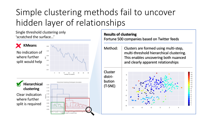
7. Clustering companies based on the company-topic matrix
Using hierarchical clustering to find meaningful groups among companies. Clusters are formed using multi-step, multi-threshold mechanism, which enables uncovering both nuanced and clearly apparent relationships.
To understand the results of hierarchical clusters, one has to understand the usage of dendograms (i.e. the charts below). Starting from the left, each vertical line identifies an additional cluster as we move to the right. Depending on the chosen threshold (i.e. the horizontal line) more-and-more clusters will be formed, however the number of companies’ that belong to these clusters will be smaller-and-smaller - and typically, with more clusters becoming very unevenly distributed. In the table below the charts I summarize the cluster densities for the chosen threshold.
Given that in my specific case, some clusters were demonstrating (much) stronger connections than other, I decided to use a ‘double-dip’ (my own-words…) clustering mechanism, where some selected clusters after the initial hierarchical threshold are then distributed further using a second hierarchical threshold. In my case I applied additional clustering on cluster 1 and 2 to ‘explode’ further.
In the last function in this section, I am using this ‘double-dip’ methodology to create the ‘final’ clusters for my companies.
from scipy.cluster.hierarchy import dendrogram, linkage

def fancy_dendrogram(*args, **kwargs):
    max_d = kwargs.pop('max_d', None)
    if max_d and 'color_threshold' not in kwargs:
        kwargs['color_threshold'] = max_d
    annotate_above = kwargs.pop('annotate_above', 0)

    ddata = dendrogram(*args, **kwargs)

    if not kwargs.get('no_plot', False):
        plt.title('Hierarchical Clustering Dendrogram (truncated)')
        plt.xlabel('sample index or (cluster size)')
        plt.ylabel('distance')
        for i, d, c in zip(ddata['icoord'], ddata['dcoord'], ddata['color_list']):
            x = 0.5 * sum(i[1:3])
            y = d[1]
            if y > annotate_above:
                plt.plot(x, y, 'o', c=c)
                plt.annotate("%.3g" % y, (x, y), xytext=(0, -5),
                             textcoords='offset points',
                             va='top', ha='center')
        if max_d:
            plt.axhline(y=max_d, c='k')
    return ddata
def plot_hierarchical_cluster(company_topic_matrix,max_d):
data=np.matrix(company_topic_matrix.Tweet_Topics.tolist())
Z = linkage(data, 'ward')
fancy_dendrogram(
Z,
truncate_mode='lastp',
p=30,
leaf_rotation=90.,
leaf_font_size=12.,
show_contracted=True,
annotate_above=10,
max_d=max_d,
)
plt.show()def hierarchy_freq_table(clusters):
df_c = pd.DataFrame(clusters,columns=['Cluster']).Cluster
df_c = df_c.value_counts().sort_index().reset_index().merge(df_c.value_counts(normalize=True).mul(100).round(1).reset_index(),on='index')
df_c.columns=['clusters','#_comp','%_comp']
return df_cmax_d = 0.1
plt.rcParams['figure.figsize'] = [7, 5]
plot_hierarchical_cluster(company_topic_matrix,max_d)
main_clusters = hierarchical_cluster(company_topic_matrix,max_d)
hierarchy_freq_table(main_clusters)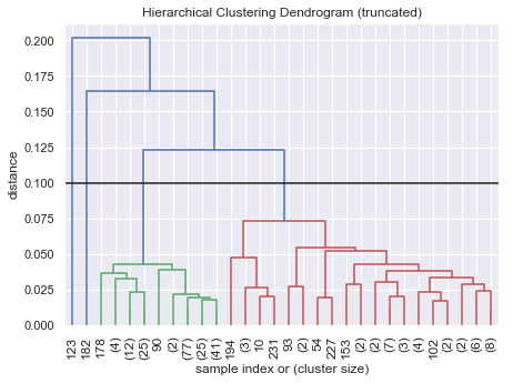
Found 4 clusters
| clusters | #_comp | %_comp | |
|---|---|---|---|
| 0 | 1 | 188 | 78.7 |
| 1 | 2 | 49 | 20.5 |
| 2 | 3 | 1 | 0.4 |
| 3 | 4 | 1 | 0.4 |
max_d = 0.0185
c = 1

df_dive = cluster_dip(company_topic_matrix, main_clusters, c)
plot_hierarchical_cluster(df_dive,max_d)
hierarchy_freq_table(hierarchical_cluster(df_dive,max_d))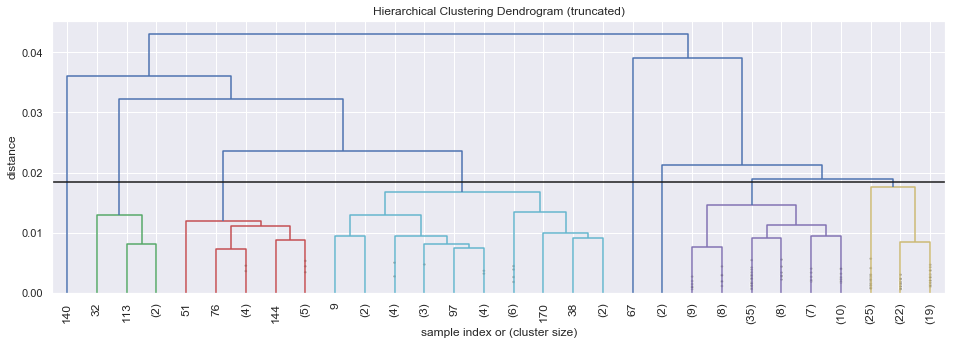
Found 8 clusters
| clusters | #_comp | %_comp | |
|---|---|---|---|
| 0 | 1 | 4 | 2.1 |
| 1 | 2 | 12 | 6.4 |
| 2 | 3 | 25 | 13.3 |
| 3 | 4 | 1 | 0.5 |
| 4 | 5 | 2 | 1.1 |
| 5 | 6 | 77 | 41.0 |
| 6 | 7 | 66 | 35.1 |
| 7 | 8 | 1 | 0.5 |
max_d = 0.035
c = 2

df_dive = cluster_dip(company_topic_matrix, main_clusters, c)
plot_hierarchical_cluster(df_dive,max_d)
hierarchy_freq_table(hierarchical_cluster(df_dive,max_d))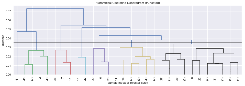
Found 7 clusters
| clusters | #_comp | %_comp | |
|---|---|---|---|
| 0 | 1 | 5 | 10.2 |
| 1 | 2 | 1 | 2.0 |
| 2 | 3 | 3 | 6.1 |
| 3 | 4 | 2 | 4.1 |
| 4 | 5 | 3 | 6.1 |
| 5 | 6 | 12 | 24.5 |
| 6 | 7 | 23 | 46.9 |
def cluster_dip(company_topic_matrix, clusters, cluster_num):
    company_topic_cluster = pd.concat([company_topic_matrix,pd.DataFrame(clusters,columns=['Cluster'])],axis=1)
    company_topic_cluster = company_topic_cluster[company_topic_cluster.Cluster==cluster_num].drop(['Cluster'],axis=1)
    return company_topic_cluster

def hierarchical_cluster(company_topic_matrix,max_d):
    from scipy.cluster.hierarchy import fcluster

    data=np.matrix(company_topic_matrix.Tweet_Topics.tolist())
    Z = linkage(data, 'ward')

    clusters = fcluster(Z, max_d, criterion='distance')
    print(f'Found {np.unique(clusters).shape[0]} clusters')

    return clusters

def cluster_deep_dive(array_doc_topics, array_companies, array_clusters, list_topic_names, list_dive_into_clusters=None, list_dive_into_maxd=None, bool_rescale=True):

    # Create dataframe from companies and topic model output 'topics'
    # Then groupby company and average topic vectors into 1 list per company
    list_company_topic_matrix = (pd.DataFrame(list(zip(array_companies,
                                                       array_doc_topics)),
                                              columns=['Company','Tweet_Topics'])
                            .groupby(['Company'])['Tweet_Topics']
                            .apply(lambda x: np.mean(np.array(x),axis=0))
                            .reset_index()
                           )

    # Explode the 1 list per company into a matrix style dataframe
    array_topic_matrix = pd.DataFrame(list_company_topic_matrix.Tweet_Topics.tolist()).values

    # If bool_rescale is True, rescale vectors (0,1)
    if bool_rescale:
        min_max_scaler = MinMaxScaler()
        array_topic_matrix = min_max_scaler.fit_transform(array_topic_matrix)

    # Create company-topics-cluster dataframe with named topics
    df_company_topic_cluster = pd.concat([list_company_topic_matrix.Company,
                    pd.DataFrame(array_topic_matrix,columns=topic_names),
                    pd.DataFrame(array_clusters,columns=['Cluster'])
                   ],axis=1)
    #df_company_topic_cluster['Orig_Clusters'] = df_company_topic_cluster['Cluster']

    # Re-cluster selected clusters
    if list_dive_into_clusters is not None:

        # Loop through each cluster to be broken up
        for i, cluster_num in enumerate(list_dive_into_clusters):

            print('*'*50)
            print(f'Working on passed cluster_id {cluster_num}')

            # Extract max_d
            max_d = list_dive_into_maxd[i]

            # Take data for deep-dive cluster and re-cluster
            df_deepdive_company_topics_cluster = cluster_dip(list_company_topic_matrix, array_clusters, cluster_num)
            array_deep_dive_clusters = hierarchical_cluster(df_deepdive_company_topics_cluster,max_d)
            df_deepdivecompany_newtopic = pd.concat([df_deepdive_company_topics_cluster.reset_index(),
                                                     pd.DataFrame(array_deep_dive_clusters,
                                                                  columns=['Cluster'])],axis=1)

            # Append new cluster to original
            df_company_topic_cluster = (df_company_topic_cluster
                                         .merge(df_deepdivecompany_newtopic, how='left',left_index=True,right_on='index')
                                         .drop(['index','Company_y','Tweet_Topics'],axis=1)
                                        )
            # Rename weird merge names
            df_company_topic_cluster.rename({'Company_x': 'Company',
                        'Cluster_x': 'Cluster_Main',
                        'Cluster_y': 'Cluster_deepdive'},
                       axis = 1, inplace=True)

            # Create temporary merged clusters
            df_company_topic_cluster['Cluster_Main'] = np.where(
                np.isnan(df_company_topic_cluster['Cluster_deepdive'])==False,
                df_company_topic_cluster['Cluster_Main'].astype(str)+df_company_topic_cluster['Cluster_deepdive'].astype(str),
                df_company_topic_cluster['Cluster_Main'].astype(str))

            # Create mapping table for new clusters
            d=defaultdict(str)
            new_c = range(1,df_company_topic_cluster.Cluster_Main.nunique()+1)
            d_i = 0
            for c in df_company_topic_cluster.Cluster_Main.unique():
                if not d[c]:
                    d[c]=new_c[d_i]
                    d_i += 1

            # Re-map clusters based on mapping table
            df_company_topic_cluster['Cluster'] = df_company_topic_cluster['Cluster_Main'].map(d)

            # Re-set index
            df_company_topic_cluster.reset_index(inplace=True)

            # Delete new columns to make table look like in the beginning
            del df_company_topic_cluster['Cluster_deepdive']
            del df_company_topic_cluster['Cluster_Main']
            del df_company_topic_cluster['index']
            #print(df_company_topic_cluster.index)

return df_company_topic_clustertweet_string, nmf_doc_topics, company_topic_matrix = read_from_saved_model(saved_model='20181113-140709_nmf_15.sav')array_doc_topics = nmf_doc_topics
array_companies = [c for c,_ in tweet_string]
array_clusters = hierarchical_cluster(company_topic_matrix,0.12)
list_topic_names = ['0-Problem_send_more_info','1-Enjoy_Our_Savings','2-Issue_Shoutout','3-Wrong_Company','4-CustomerCare_Will_Help','5-Future',
'6-Problem_Do_A_Claim','7-Apologies','8-Appreciation','9-Media_Queries','10-Store_Feedback',
'11-Payments','12-Community','13-Problem_Followup_on_Claim','14-Problem_Direct_Message'
]
list_dive_into_clusters = [1,2]
list_dive_into_maxd = [0.0185,0.035]
bool_rescale = True
df = cluster_deep_dive(array_doc_topics, array_companies, array_clusters, list_topic_names, list_dive_into_clusters, list_dive_into_maxd, bool_rescale)Found 4 clusters
**************************************************
Working on passed cluster_id 1
Found 8 clusters
**************************************************
Working on passed cluster_id 2
Found 7 clusters
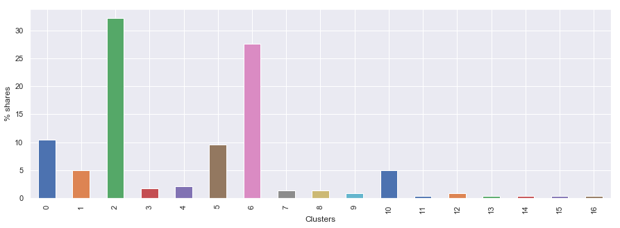
8. Visualizing clustering results
Frequency table
As a first viz I am showing the cluster frequency diagram.
ax = hierarchy_freq_table(df.Cluster)['%_comp'].plot(kind='bar',figsize=(15, 5))
ax.set_xlabel('Clusters')
ax.set_ylabel('% shares')
Text(0, 0.5, '% shares')
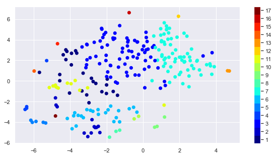
TSNE charts
As a second viz I am showing a (custom) TSNE chart to bring the multi-dimensional problem into 2-dimensions (i.e. x-y axes). This graph shows that the identified clusters (shows as colors) are not far from each other in distance on the chart, where distance between points ABSTRACTLY represents the strenght of relationship between the elements (note: TSNE charts are almost impossible to interpret, the key thing is that same colors should not be too distributed from each other).
from sklearn.manifold import TSNE
plt.rcParams['figure.figsize'] = [10, 5]

time_start = time()

data=np.matrix(company_topic_matrix.Tweet_Topics.tolist())

tsne = TSNE(n_components=2, verbose=1, perplexity=70, n_iter=5000)
tsne_pca_results = tsne.fit_transform(data)

df_tsne = None
df_tsne = pd.DataFrame(df.Cluster)
df_tsne['x-tsne-pca'] = tsne_pca_results[:,0]
df_tsne['y-tsne-pca'] = tsne_pca_results[:,1]

print('t-SNE done! Time elapsed: {} seconds'.format(time()-time_start))

plt.scatter(df_tsne['x-tsne-pca'], df_tsne['y-tsne-pca'], c=df_tsne['Cluster'], cmap=plt.cm.get_cmap("jet", df_tsne['Cluster'].nunique()))
plt.colorbar(ticks=range(1,df_tsne['Cluster'].nunique()+1))
plt.clim(0.5, df_tsne['Cluster'].nunique()+0.5)
plt.show()
[t-SNE] Computing 211 nearest neighbors...
[t-SNE] Indexed 239 samples in 0.000s...
[t-SNE] Computed neighbors for 239 samples in 0.012s...
[t-SNE] Computed conditional probabilities for sample 239 / 239
[t-SNE] Mean sigma: 0.002370
[t-SNE] KL divergence after 250 iterations with early exaggeration: 51.601948
[t-SNE] KL divergence after 1100 iterations: 0.291489
t-SNE done! Time elapsed: 2.903787851333618 seconds
Simple listing
As a very simple summary, I am printing the identified cluster for each of the companies. Some interesting groups are already visible
for name, values in df[['Company','Cluster']].groupby('Cluster'):
    v=', '.join(values.Company.tolist())
    print(f'Cluster: {name}: {v}')
    print()
Cluster: 1: 3M, Adobe, Aetna, Ally, CapitalOne, Cummins, DRHorton, Dillards, Discover, GapInc, HormelFoods, JohnDeere, LibertyMutual, MolsonCoors, MurphyUSA, Nationwide, Sysco, Target, Voya, WaldorfAstoria, Walmart, honeywell, keybank, lincolnfingroup, oreillyauto
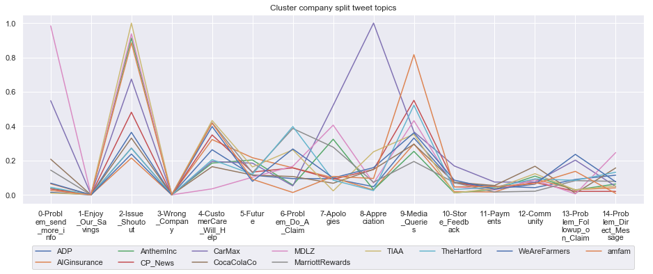
Cluster: 2: ADP, AIGinsurance, AnthemInc, CP_News, CarMax, CocaColaCo, MDLZ, MarriottRewards, TIAA, TheHartford, WeAreFarmers, amfam
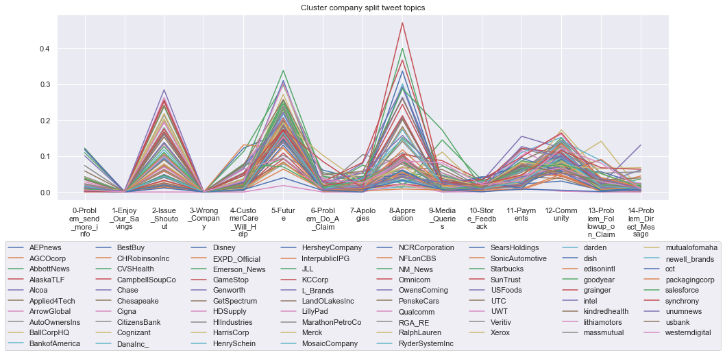
Cluster: 3: AEPnews, AGCOcorp, AbbottNews, AlaskaTLF, Alcoa, Applied4Tech, ArrowGlobal, AutoOwnersIns, BallCorpHQ, BankofAmerica, BestBuy, CHRobinsonInc, CVSHealth, CampbellSoupCo, Chase, Chesapeake, Cigna, CitizensBank, Cognizant, DanaInc_, Disney, EXPD_Official, Emerson_News, GameStop, Genworth, GetSpectrum, HDSupply, HIIndustries, HarrisCorp, HenrySchein, HersheyCompany, InterpublicIPG, JLL, KCCorp, L_Brands, LandOLakesInc, LillyPad, MarathonPetroCo, Merck, MosaicCompany, NCRCorporation, NFLonCBS, NM_News, Omnicom, OwensCorning, PenskeCars, Qualcomm, RGA_RE, RalphLauren, RyderSystemInc, SearsHoldings, SonicAutomotive, Starbucks, SunTrust, USFoods, UTC, UWT, Veritiv, Xerox, darden, dish, edisonintl, goodyear, grainger, intel, kindredhealth, lithiamotors, massmutual, mutualofomaha, newell_brands, oct, packagingcorp, salesforce, synchrony, unumnews, usbank, westerndigital
Cluster: 4: AdvanceAuto, Chevron, Publix, caseysgenstore
Cluster: 5: Albertsons, DICKS, Lowes, kroger, riteaid
Cluster: 6: Allstate, AmericanAir, BBT, BedBathBeyond, ConagraBrands, DellTech, Delta, DukeEnergy, FrontierCorp, GeneralMills, Hanes, JetBlue, Kohls, KraftHeinzCo, Lennar, Nordstrom, SouthwestAir, StateFarm, XcelEnergyCO, erie_insurance, firstenergycorp, footlocker, generalelectric
Cluster: 7: AltriaNews, AmericanAxle, Amgen, Anixter, Aramark, Avnet, CDWCorp, CSX, CalpineCareers, Celgene, Corning, DXCTechnology, DaVita, EastmanChemCo, Ecolab, FISGlobal, FluorCorp, GoldmanSachs, Graybar, HPE, Halliburton, Huntsman_Corp, IntlPaperCo, JNJNews, LamResearch, LasVegasSands, LearCorporation, LeidosInc, LockheedMartin, MMC_Global, ManpowerGroup, McKesson, Microsoft, MorganStanley, MotoSolutions, NOVGlobal, Newmont, Oracle, PPG, ROKAutomation, RaymondJames, Raytheon, SanminaCorp, SouthernCompany, TXInstruments, TysonFoods, UnitedHealthGrp, United_Rentals, Univar, WestRock, WhirlpoolCorp, WilliamsUpdates, abbvie, airproducts, baxter_intl, biogen, blackrock, blackstone, bmsnews, cardinalhealth, conocophillips, exxonmobil, kiewit, nvidia, thermofisher, zimmerbiomet
Cluster: 8: Assurant, RepublicService, XPOLogistics
Cluster: 9: AutoNation, DollarGeneral, InsidePMI
Cluster: 10: DTE_Energy, officedepot
Cluster: 11: DrPepperSnapple, FedEx, HP, KelloggCompany, NAPAKnowHow, Progressive, Prudential, Thrivent, Travelers, WellsFargo, molinahealth, principal
Cluster: 12: HomeDepot
Cluster: 13: McDonaldsCorp, PepsiCo
Cluster: 14: MetLife
Cluster: 15: Visa
Cluster: 16: WarnerMediaGrp
Cluster: 17: autozone
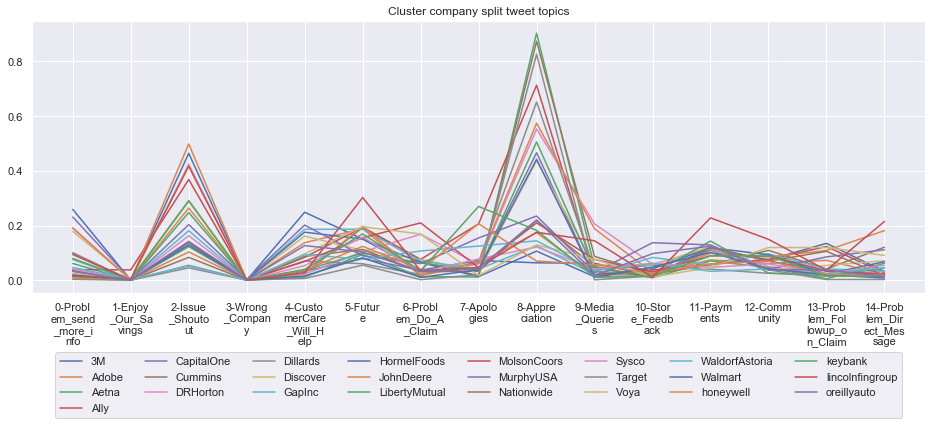
Detailed cluster analyis
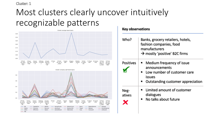
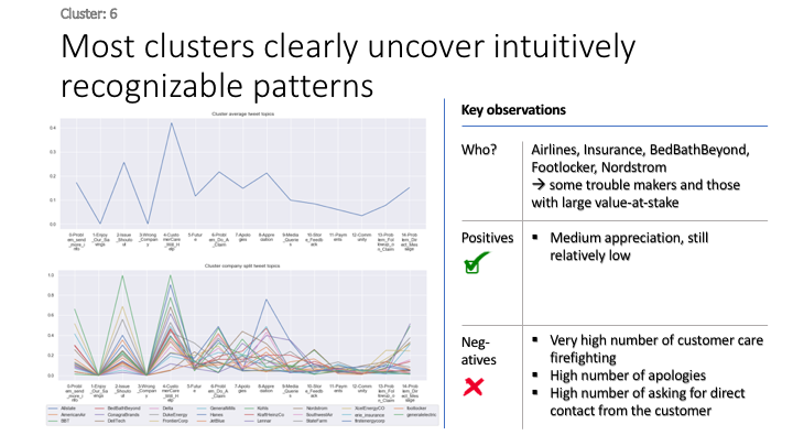
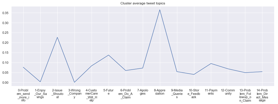
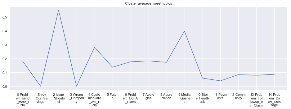
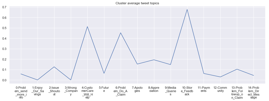
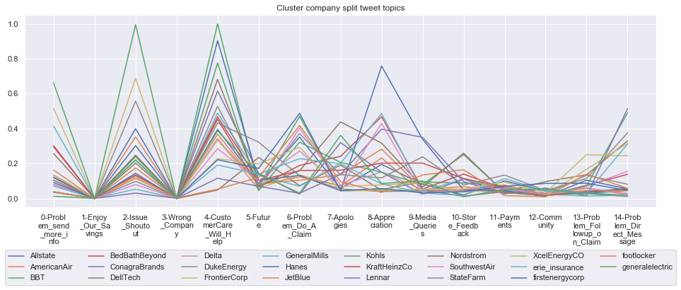
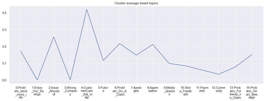
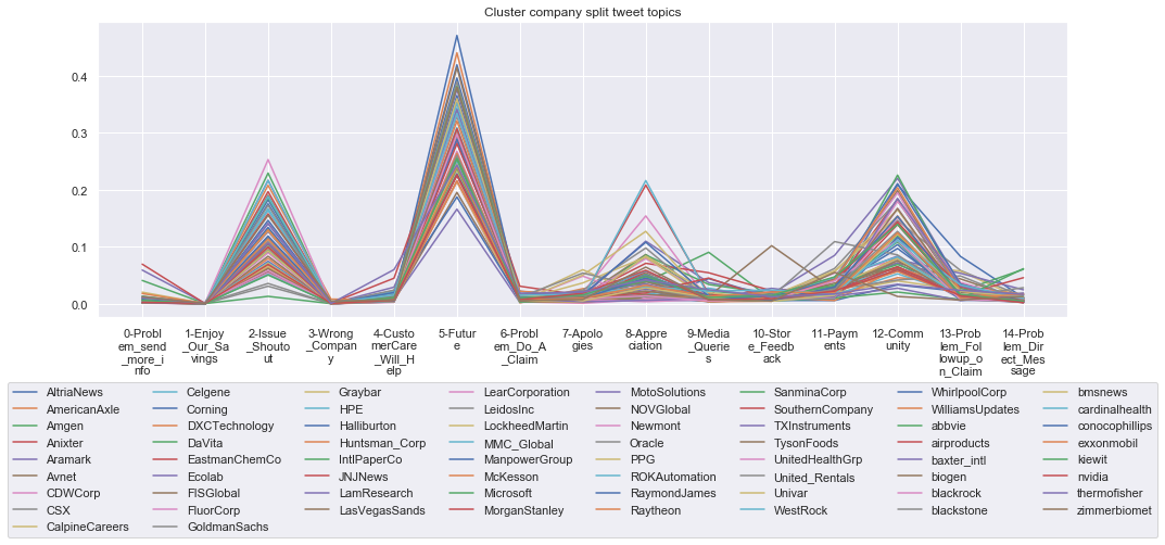
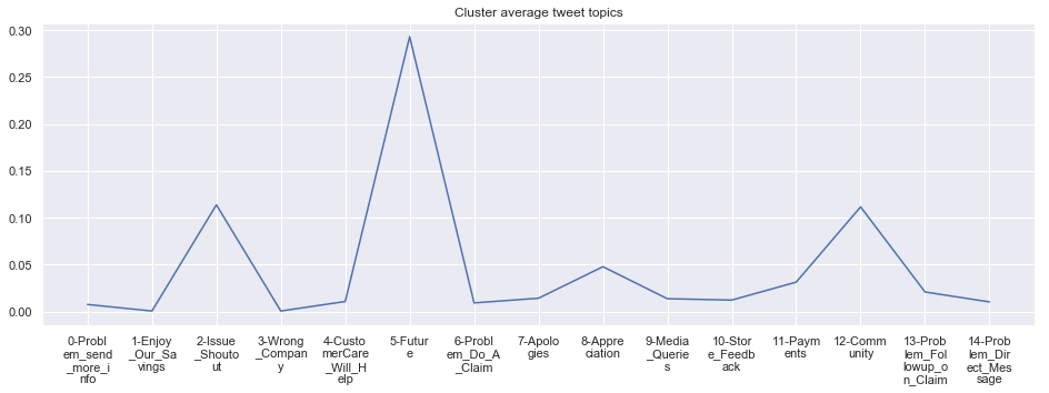
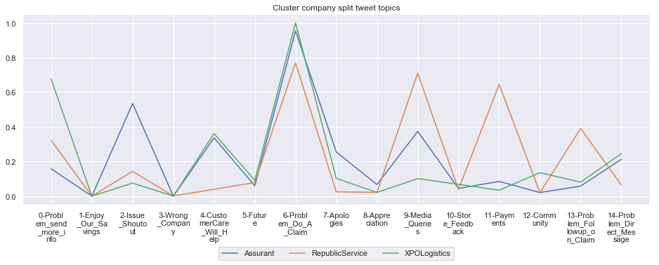
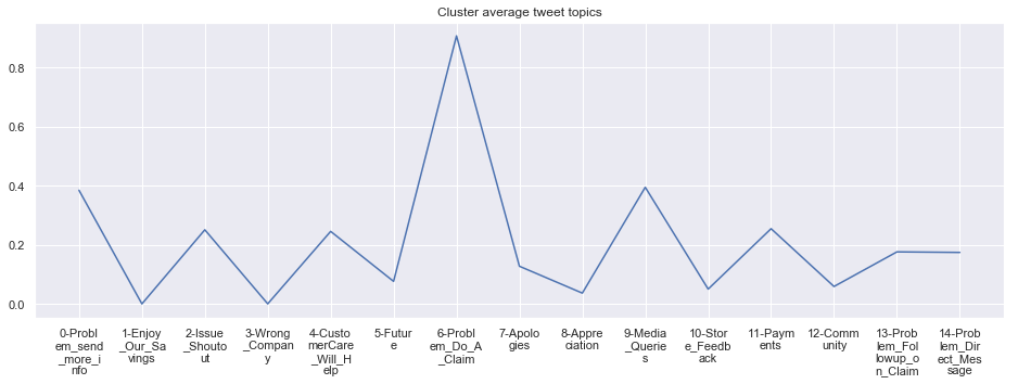
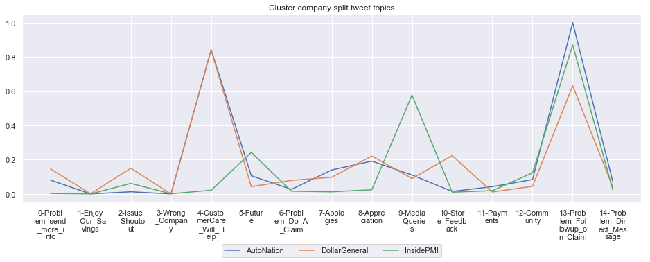
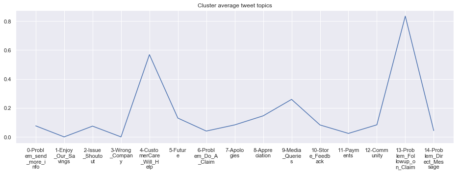
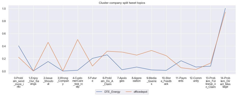
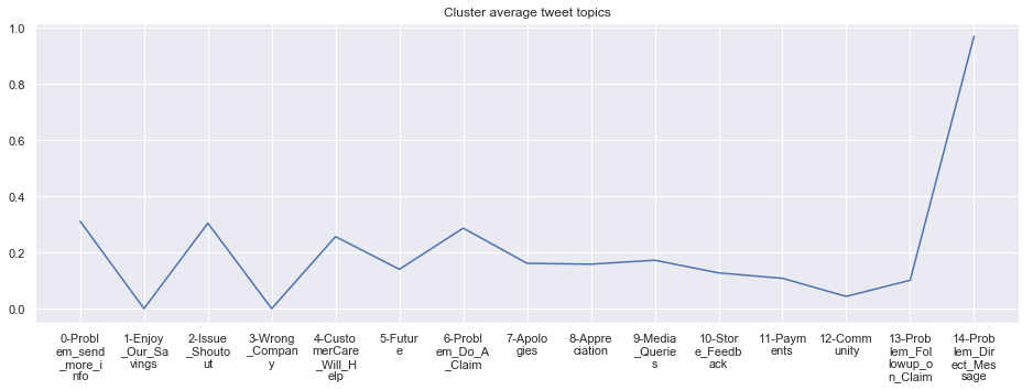
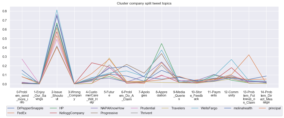
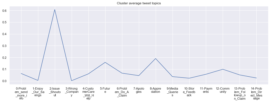
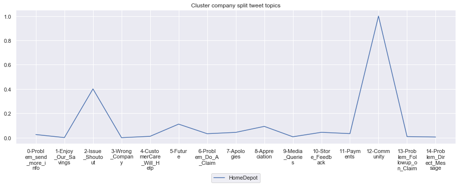
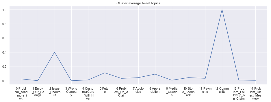
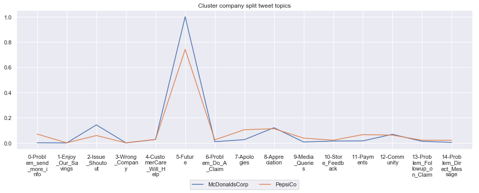
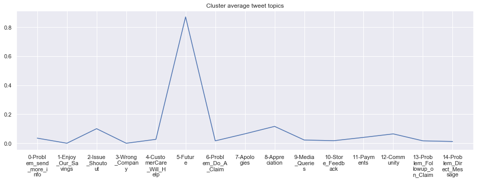
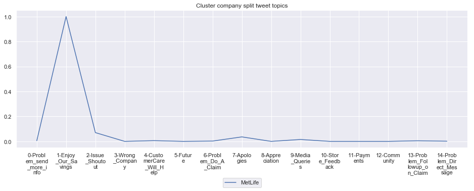
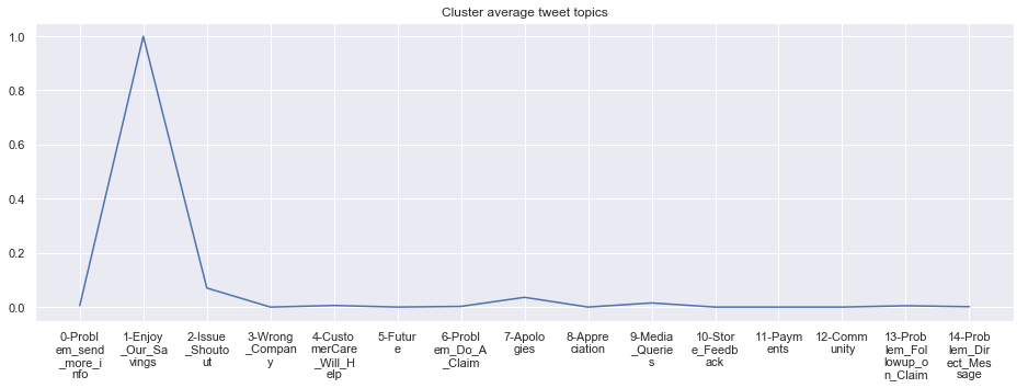
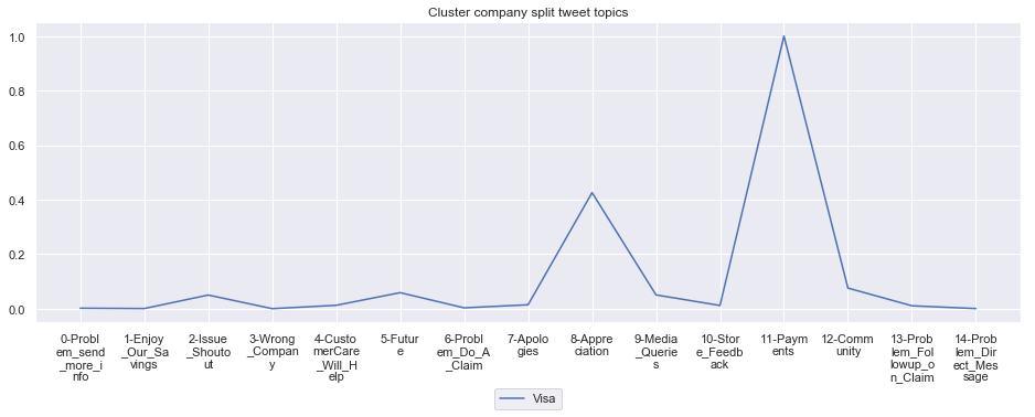
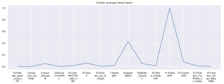
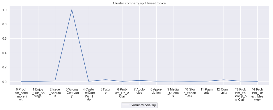
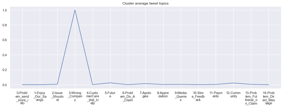
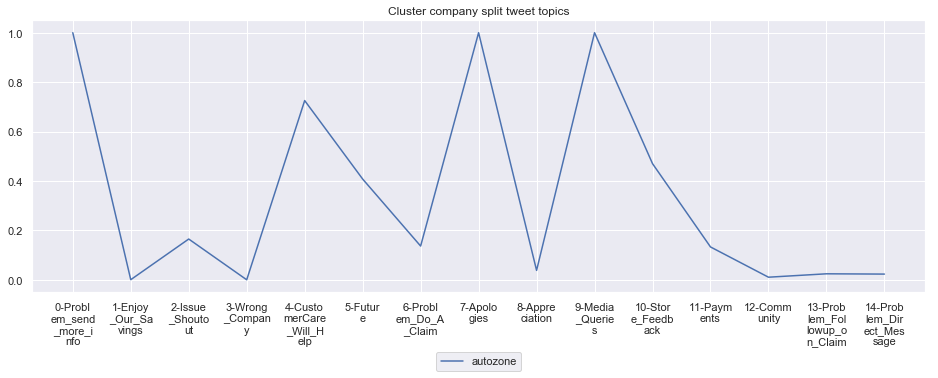
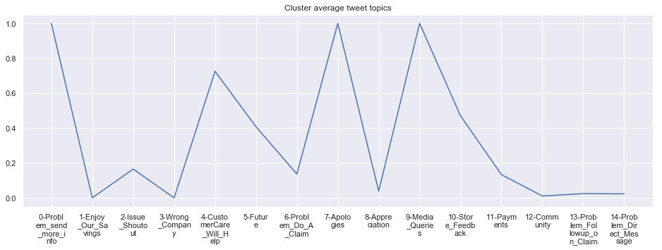
To give more flavour to the clustering viz, the below charts show cluster-by-cluster the companies that belong there (lines) and the relative topic-frequency along which each company has tweeted in the past 1000 tweets.
This technique enables us to understand the basis of the clusters (based on the topics), have a closer look which companies ended up together, and infer some potentially present business relationships, e.g. airlines ended up in cluster 6, and they tend to use Twitter mainly for customer-service. Whereas some other companies use it more to publish some ideas about the future, or to just simply praise their customers.
grouped = df.groupby('Cluster')
plt.rcParams['figure.figsize'] = [16, 5]
font = {'size'   : 22}
plt.rc('font', **font)

cluster_average = grouped[df.columns[1:-1]].agg('mean').reset_index()
cluster_average_cleaned = cluster_average.drop(['Cluster'],axis=1).T


for name, group in grouped:

    print('*'*54,f'Cluster {name}','*'*54)
    #print(np.array(group.Company))
    group.drop(['Cluster'],axis=1).T.iloc[1:].plot(legend=None)
    #print(group.T.index[1:-1])
    plt.xticks(range(15),['\n'.join(wrap(l, 7)) for l in group.T.index[1:-1]])
    plt.title('Cluster company split tweet topics')
    #plt.legend(group.Company)

    # Put a legend below current axis
    plt.legend(group.Company,loc='upper center', bbox_to_anchor=(0.5, -0.2),ncol=8, fancybox=True)

    plt.show()

    i = name-1
    cluster_average_cleaned[i].plot(legend=None)
    plt.xticks(range(15),['\n'.join(wrap(l, 7)) for l in cluster_average.T.index[1:]])
    plt.title('Cluster average tweet topics')
    #plt.legend(cluster_average.Cluster[i:],loc='upper center', bbox_to_anchor=(0.5, -0.2),ncol=8, fancybox=True)
    plt.show()
****************************************************** Cluster 1 ******************************************************
****************************************************** Cluster 2 ******************************************************
****************************************************** Cluster 3 ******************************************************
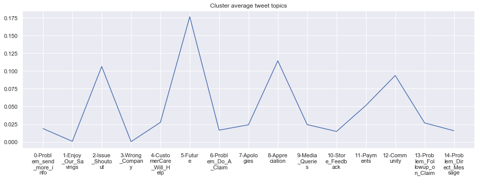
****************************************************** Cluster 4 ******************************************************
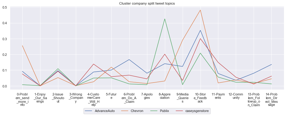
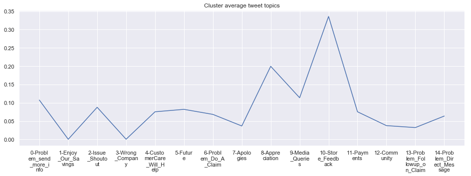
****************************************************** Cluster 5 ******************************************************
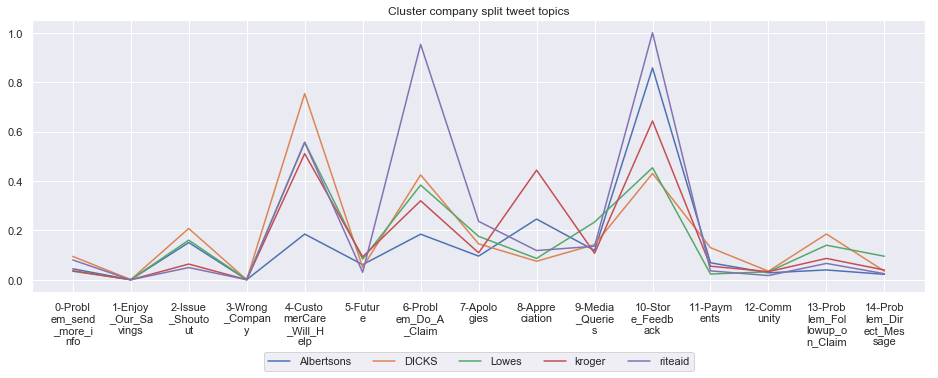
****************************************************** Cluster 6 ******************************************************
****************************************************** Cluster 7 ******************************************************
****************************************************** Cluster 8 ******************************************************
****************************************************** Cluster 9 ******************************************************
****************************************************** Cluster 10 ******************************************************
****************************************************** Cluster 11 ******************************************************
****************************************************** Cluster 12 ******************************************************
****************************************************** Cluster 13 ******************************************************
****************************************************** Cluster 14 ******************************************************
****************************************************** Cluster 15 ******************************************************
****************************************************** Cluster 16 ******************************************************
****************************************************** Cluster 17 ******************************************************
Sections not in use, but still relevant
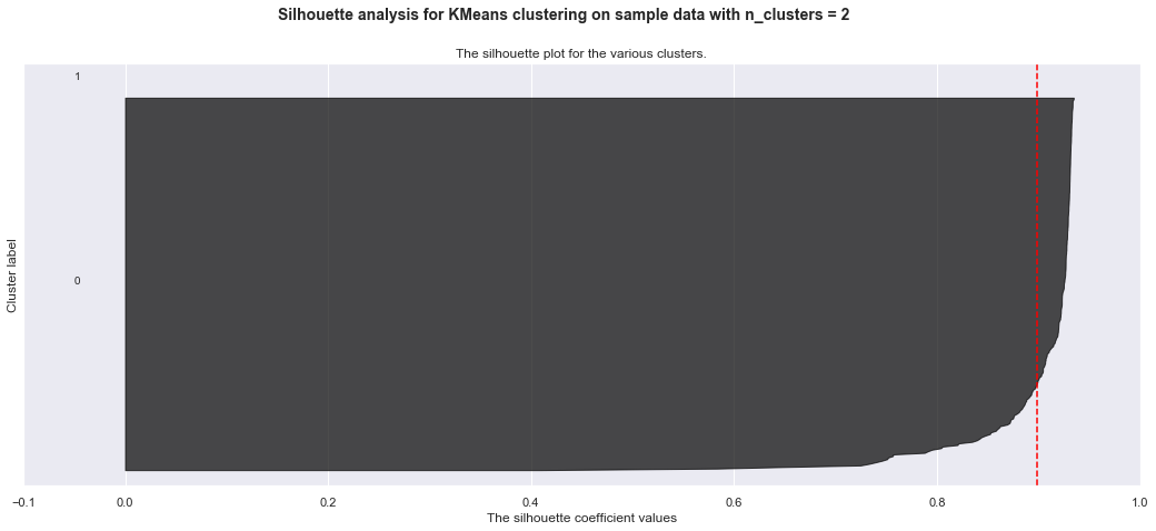
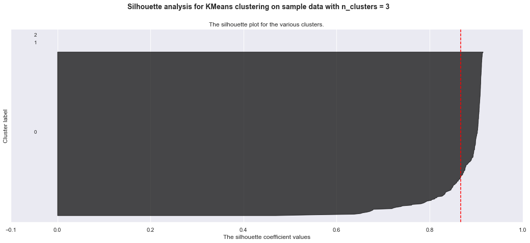
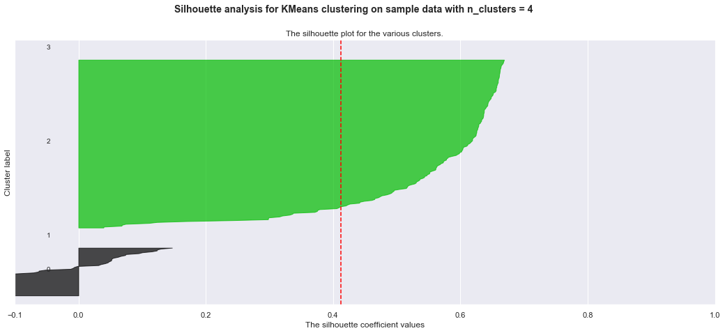
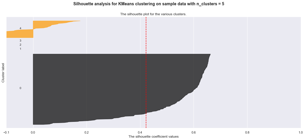
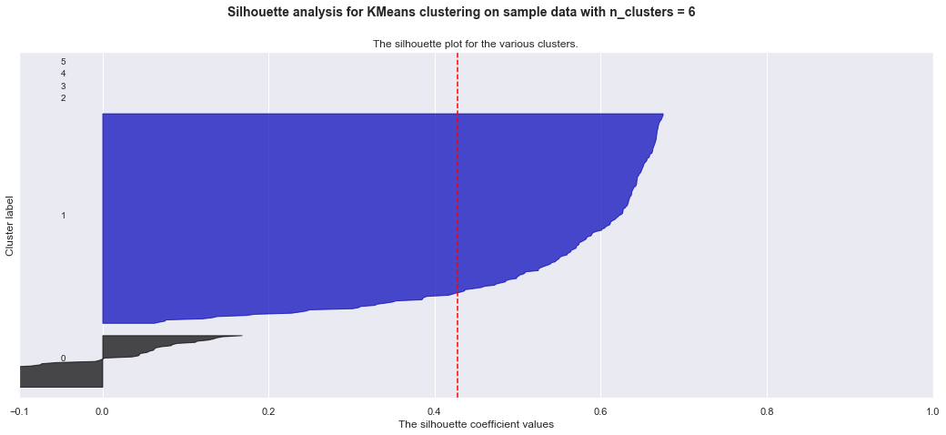
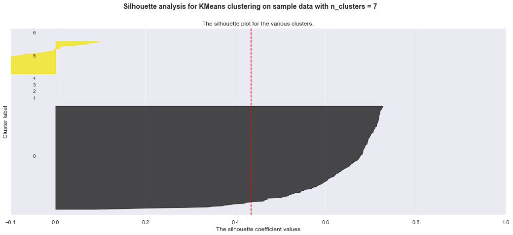
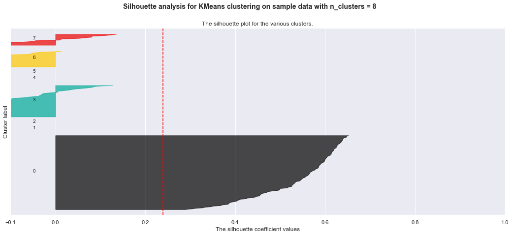
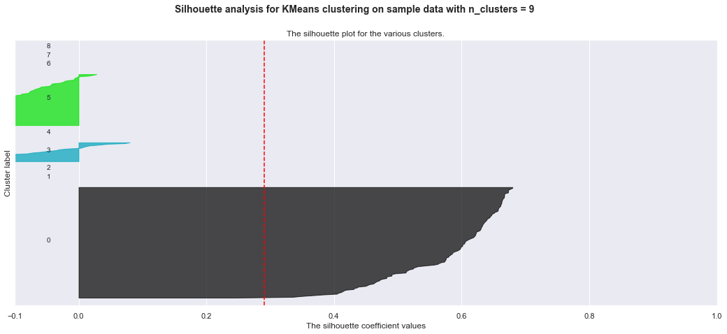
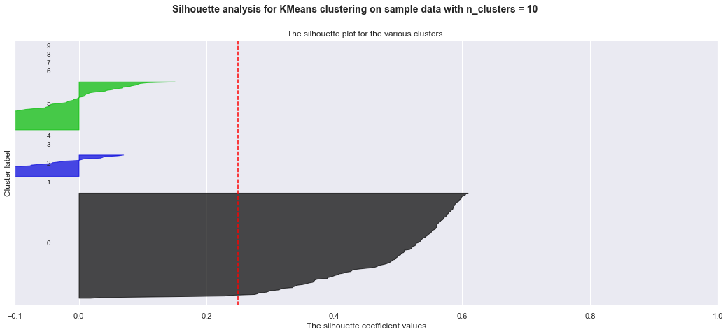
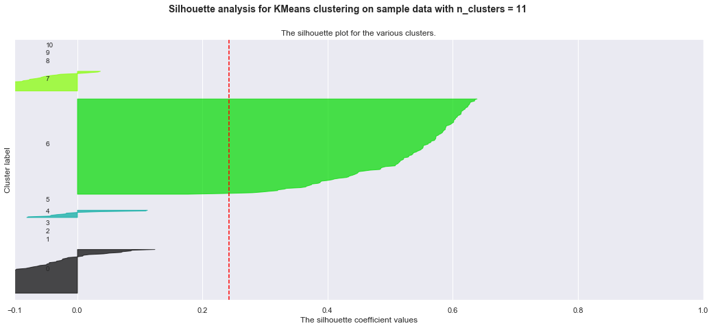
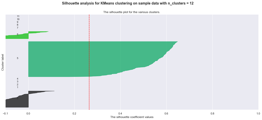
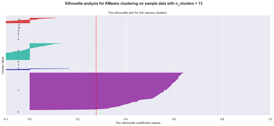
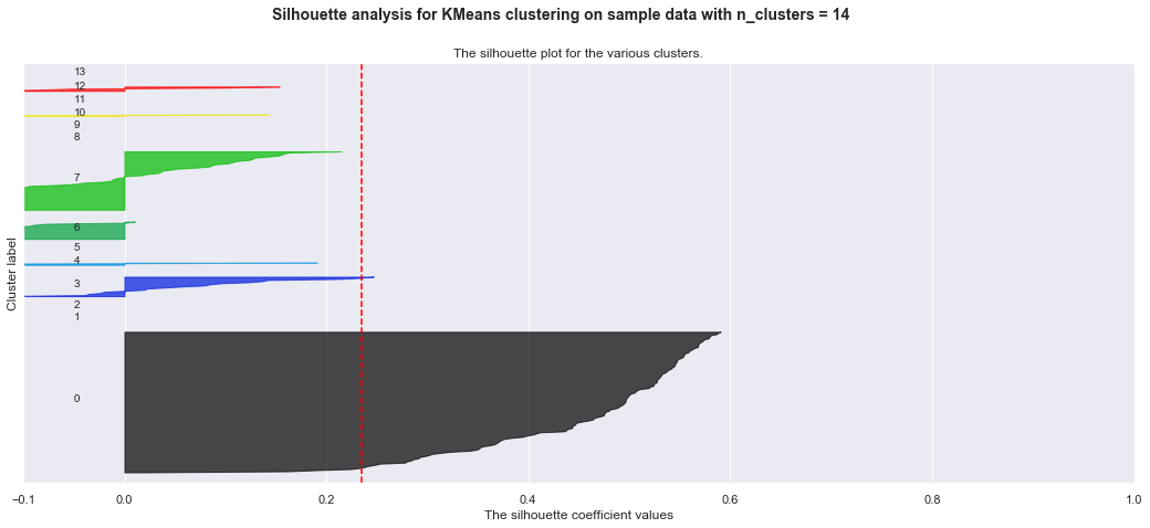
Below are my trials with KMeans clustering before I realized I want to use hierarchical clustering. The detailed silhoutte analysis shows the weak clusters identified.
# Clustering: KMeans
from sklearn.cluster import MiniBatchKMeans
km = MiniBatchKMeans(n_clusters=13)
km.fit(np.matrix(company_topic_matrix.Tweet_Topics.tolist()))
MiniBatchKMeans(batch_size=100, compute_labels=True, init='k-means++',
init_size=None, max_iter=100, max_no_improvement=10, n_clusters=13,
n_init=3, random_state=None, reassignment_ratio=0.01, tol=0.0,
verbose=0)
unique, counts = np.unique(km.labels_, return_counts=True)
total = np.sum(counts)
print(np.asarray((unique, counts/total*100)).T)
[[ 0. 1.25523013]
[ 1. 56.90376569]
[ 2. 0.41841004]
[ 3. 0.41841004]
[ 4. 5.43933054]
[ 5. 2.09205021]
[ 6. 1.25523013]
[ 7. 2.51046025]
[ 8. 1.25523013]
[ 9. 20.92050209]
[10. 0.41841004]
[11. 6.27615063]
[12. 0.83682008]]
def n_clusters_check(data):
    SSEs = []
    Sil_coefs = []
    for k in range(2,40):
        km = MiniBatchKMeans(n_clusters=k, random_state=1)
        km.fit(data)
        labels = km.labels_
        Sil_coefs.append(metrics.silhouette_score(data, labels, metric='euclidean'))
        SSEs.append(km.inertia_) # The SSE is just inertia, we
                                                # could have just said km.inertia_
    return SSEs, Sil_coefs

def plot_n_clusters(data):

    SSEs, Sil_coefs = n_clusters_check(data)

    fig, (ax1, ax2) = plt.subplots(1,2, figsize=(15,5), sharex=True)
    k_clusters = range(2,40)
    ax1.plot(k_clusters, Sil_coefs)
    ax1.set_xlabel('number of clusters')
    ax1.set_ylabel('silhouette coefficient')

    # plot here on ax2
    ax2.plot(k_clusters, SSEs)
    ax2.set_xlabel('number of clusters')
    ax2.set_ylabel('SSE');
from sklearn import metrics
data = np.matrix(company_topic_matrix.Tweet_Topics.tolist())
plot_n_clusters(data)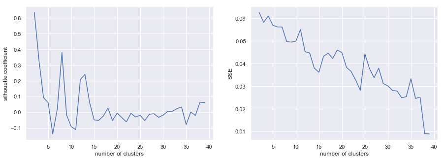
def show_variance_explained_plots(model):

    var_exp_array = model.explained_variance_ratio_
    n_comps = var_exp_array.shape[0]

    fig, ax = plt.subplots(1,2,figsize=(10,4))

    ax[0].fill_between(range(n_comps), var_exp_array)
    ax[0].set_title('Variance Explained by Nth Principal Component')

    ax[1].fill_between(range(n_comps), np.cumsum(var_exp_array))
    ax[1].set_title('Cumulative Variance Explained by N Components')

plt.show()show_variance_explained_plots(lsi_model)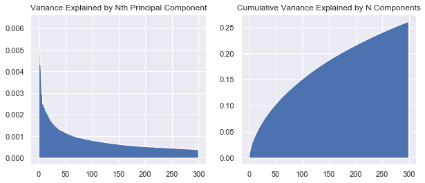
from __future__ import print_function

from sklearn.datasets import make_blobs
from sklearn.cluster import KMeans
from sklearn.metrics import silhouette_samples, silhouette_score

import matplotlib.pyplot as plt
import matplotlib.cm as cm
import numpy as np

# Generating the sample data from make_blobs
# This particular setting has one distinct cluster and 3 clusters placed close
# together.
X = data

range_n_clusters = range(2,15)

for n_clusters in range_n_clusters:
    # Create a subplot with 1 row and 2 columns
    fig, ax1 = plt.subplots(1, 1)
    fig.set_size_inches(18, 7)

    # The 1st subplot is the silhouette plot
    # The silhouette coefficient can range from -1, 1 but in this example all
    # lie within [-0.1, 1]
    ax1.set_xlim([-0.1, 1])
    # The (n_clusters+1)*10 is for inserting blank space between silhouette
    # plots of individual clusters, to demarcate them clearly.
    ax1.set_ylim([0, len(X) + (n_clusters + 1) * 10])

    # Initialize the clusterer with n_clusters value and a random generator
    # seed of 10 for reproducibility.
    clusterer = KMeans(n_clusters=n_clusters, random_state=10)
    cluster_labels = clusterer.fit_predict(X)

    # The silhouette_score gives the average value for all the samples.
    # This gives a perspective into the density and separation of the formed
    # clusters
    silhouette_avg = silhouette_score(X, cluster_labels)
    print("For n_clusters =", n_clusters,
          "The average silhouette_score is :", silhouette_avg)

    # Compute the silhouette scores for each sample
    sample_silhouette_values = silhouette_samples(X, cluster_labels)

    y_lower = 10
    for i in range(n_clusters):
        # Aggregate the silhouette scores for samples belonging to
        # cluster i, and sort them
        ith_cluster_silhouette_values = \
            sample_silhouette_values[cluster_labels == i]

        ith_cluster_silhouette_values.sort()

        size_cluster_i = ith_cluster_silhouette_values.shape[0]
        y_upper = y_lower + size_cluster_i

        color = cm.nipy_spectral(float(i) / n_clusters)
        ax1.fill_betweenx(np.arange(y_lower, y_upper),
                          0, ith_cluster_silhouette_values,
                          facecolor=color, edgecolor=color, alpha=0.7)

        # Label the silhouette plots with their cluster numbers at the middle
        ax1.text(-0.05, y_lower + 0.5 * size_cluster_i, str(i))

        # Compute the new y_lower for next plot
        y_lower = y_upper + 10  # 10 for the 0 samples

    ax1.set_title("The silhouette plot for the various clusters.")
    ax1.set_xlabel("The silhouette coefficient values")
    ax1.set_ylabel("Cluster label")

    # The vertical line for average silhouette score of all the values
    ax1.axvline(x=silhouette_avg, color="red", linestyle="--")

    ax1.set_yticks([])  # Clear the yaxis labels / ticks
    ax1.set_xticks([-0.1, 0, 0.2, 0.4, 0.6, 0.8, 1])

    plt.suptitle(("Silhouette analysis for KMeans clustering on sample data "
                  "with n_clusters = %d" % n_clusters),
                 fontsize=14, fontweight='bold')

plt.show()
For n_clusters = 2 The average silhouette_score is : 0.8986988319795822
For n_clusters = 3 The average silhouette_score is : 0.8667965252187471
For n_clusters = 4 The average silhouette_score is : 0.41195436173718575
For n_clusters = 5 The average silhouette_score is : 0.4219381410304533
For n_clusters = 6 The average silhouette_score is : 0.42767371272258947
For n_clusters = 7 The average silhouette_score is : 0.43409940385179036
For n_clusters = 8 The average silhouette_score is : 0.23933684619767728
For n_clusters = 9 The average silhouette_score is : 0.2904368838689066
For n_clusters = 10 The average silhouette_score is : 0.2488217447501851
For n_clusters = 11 The average silhouette_score is : 0.24251617076071022
For n_clusters = 12 The average silhouette_score is : 0.26415476136183297
For n_clusters = 13 The average silhouette_score is : 0.27696632549696604
For n_clusters = 14 The average silhouette_score is : 0.23469905394496227