Building a music recommendation engine

This exercise is inspired by the Music Recommendation Challenge KAGGLE competition.

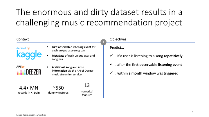
The data was provided by KKBOX, an East-Asian music streaming service, similar to Spotify. It shows the first observable listening event for each unique user-song pair, together with potenitally useful Metadata. Besides the data provided, I sourced additional song and artist information via the API of Deezer music streaming service based on a ‘real-world’ unique song identifier (ISRC id) in the KKBOX dataset

My objective utlizing classification models was to predict… …if a user is listening to a song repetitively …after the first observable listening event …within a month window was triggered

png

# Import all necessery python packages
import pandas as pd
import numpy as np
import matplotlib.pyplot as plt
import matplotlib.dates as mdates
import time
import seaborn as sns
from collections import defaultdict
import statsmodels.api as sm
import statsmodels.formula.api as smf
import swifter
from math import ceil
import pickle as pkl

from sklearn.linear_model import LogisticRegression
from sklearn.preprocessing import StandardScaler
from sklearn.metrics import fbeta_score, confusion_matrix
from sklearn.ensemble import RandomForestClassifier
import xgboost as xgb

from IPython.display import Image
%matplotlib inline

png

1. Read in the data

The data is available on via the KAGGLE here, you may have to register if you are not a member yet - it is free of charge.

By the way, KAGGLE is a really interesting source and platform to practice data science problems, and to acquire data. I highly recommend it!

KAGGLE data

def read_in_data(sample):
    '''
    
    Reads in data from music_data folder in pickle format. If sample arguement is True, it limits each df to 1000
    randomly sampled rows.
    
    input: None
    output: df_train, df_members, df_full_songs
    '''
    
    # Limiting the data to 1000 records from each db
    df_train = pd.read_pickle('./music_data/train.pkl')
    df_members = pd.read_pickle('./music_data/members.pkl')
    df_full_songs = pd.read_pickle('./music_data/df_full_songs.pkl')
    
    if sample:
        df_train = df_train.sample(1000)
        df_members = df_members.sample(1000)
        df_full_songs = df_full_songs.sample(1000)
    
    return df_train, df_members, df_full_songs

Deezer data

def downloader(df_merged):
    '''
    Download data from deezer

    input: df_merged
    otuput: dict containing the API download data
    '''

    BASE_URL = 'https://api.deezer.com/2.0/track/isrc:'
    unique_isrc = df_merged['isrc'].unique()
    total = len(unique_isrc)
    from IPython.display import clear_output, display

    for i, isrc in enumerate(unique_isrc):
        if not dict[str(isrc)]:
            clear_output(wait=True)
            try:            
                api_call = BASE_URL + str(isrc)
                r = req.get(api_call).content
                dict[str(isrc)] = r
                print('Saved:',str(isrc),i,'of',total)
            except:
                print('***Failed:***',str(isrc),i,'of',total)
                downloader(df_merged)

def save_deezer_to_pickle(dict):
    '''
    input: dict with downloaded deezer api info
    output: none, saves dict to pickle
    '''    
    # Save the downloaded data to a pkl file
    with open('deezer_data.pkl', 'wb') as handle:
        pickle.dump(dict, handle, protocol=pickle.HIGHEST_PROTOCOL)
        
def deezer_into_df(dict):    
    '''
    Take the dict with the downloaded API data

    input: dict with downloaded api info
    output: df_isrc in memory and saved to disk, containing the useful info from 

    '''
    import json
    dfs=[]
    for key, value in dict.items():
        json1_data = json.loads(value)

        try:
            isrc_query = np.array([
                key,
                json1_data['title'],
                json1_data['album']['title'],
                json1_data['artist']['name'],
                json1_data['release_date'],
                json1_data['duration'],
                json1_data['track_position'],
                json1_data['bpm'],
                json1_data['gain'],
                json1_data['rank']
                                  ])
            df_isrc_query = pd.DataFrame(isrc_query.reshape(1,isrc_query.size))
            dfs.append(df_isrc_query)
        except:
            try:
                if json1_data['error']['code'] == 800:
                    pass #all response 800 just pass
            except:
                print(key,'/n', json1_data)
                pass
    df_isrc_all = pd.concat(dfs)
    df_isrc_all.columns = ['isrc','track_title','album_title','artist_name','release_date','duration_sec','track_pos','bpm','gain','rank']
    df_isrc_all.reset_index(inplace=True)
    del df_isrc_all['index']
    df_isrc_all.to_pickle('df_isrc.pkl')
    
    return df_isrc_all

Merging deezer and kaggle data

def create_df_full_songs(df_song_extra,df_songs,df_isrc):
    '''
    Merging the relationally stored sub-tables that describe the metadata for each song into a single table
    
    input: df_song_extra,df_songs,df_isrc
    output: df_full_songs
    '''
    
    df_song_extra = pd.read_pickle('./music_data/song_extra_info.pkl')
    df_songs = pd.read_pickle('./music_data/songs.pkl')
    df_isrc = pd.read_pickle('./music_data/df_isrc.pkl')

    # To analyze song data, I am merging df_songs, df_songs_extra and df_isrc
    df_full_songs = (df_songs
                 .merge(df_songs,on='song_id',how='left')
                 .merge(df_song_extra,on='isrc',how='left')
                )

    # Deleting song data elements to save memory. Everything saved under df_full_songs
    del df_song_extra
    del df_songs
    del df_isrc

    # Write df_full_songs
    df_full_songs.to_pickle('./music_data/df_full_songs.pkl')

    return df_full_songs

2. Feature engineering

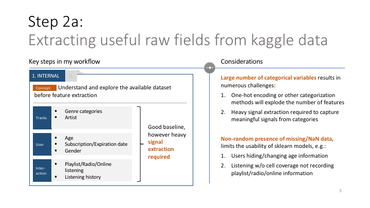
On each of the provided tables I am extracting signals that could direct the classifier model to be built later. This is a crucial step in machine learning, and as I learned spending 80% of your time on feature engineering and 20% on model training is usually a good balance.

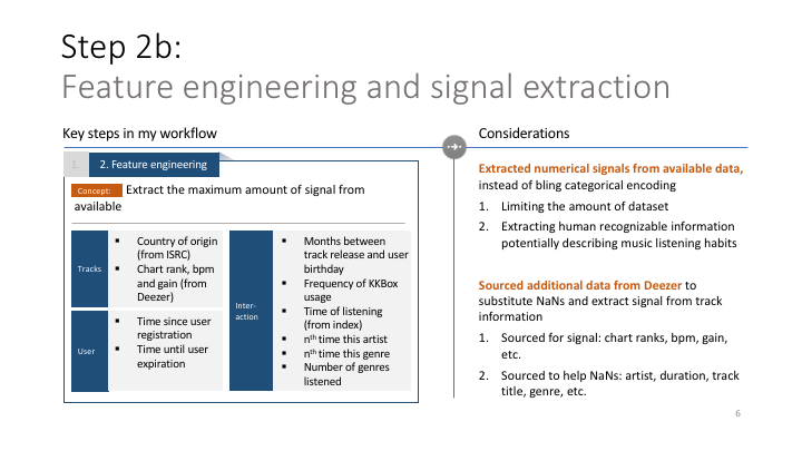
As the data (likely) was originally stored in relational databases at KKBOX, KAGGLE provided it each logical piece of information in separate files. Below I am extracting the features individually from the tables where possible, once done I am merging the tables and extract signals, from the merged (unique song-user combos) table.

Side comment: as you may see, I am using pickle to save and load databases across my work on this blog. Pickle is a fast and easy alternative to csv, it can hold all types of data I came across (including saved neural network models with some tweaking) and it is much faster than csv in cases I observed.

png png png

def full_songs_engineering(df_full_songs):
    '''
    input: df_full_songs
    output: df_full_songs cleaned and engineered
    '''
    
    # Extract country of origin from isrc
    df_full_songs['song_language_isrc'] = np.where(df_full_songs['isrc'].isna(),
                                                   np.NaN,
                                                   df_full_songs['isrc'].astype(str).str[:2])
    
    # Count the number of genre_ids
    df_full_songs['count_genre_ids'] = df_full_songs['genre_ids'].str.count('\|')+1

    # Categorize genre (can be multiple)
    dfs=[]
    df_all_genres = pd.DataFrame(df_full_songs['genre_ids'].str.split('|',expand=True)).fillna(value=np.NaN)
    for i, column in enumerate(df_all_genres):
        dfs.append(pd.get_dummies(df_all_genres[i], prefix = 'genre_CAT'))
    df_genre_merged = pd.concat(dfs, axis=1)
    df_genre_merged = df_genre_merged.groupby(df_genre_merged.columns, axis=1).agg(np.max)
    df_full_songs = pd.concat([df_full_songs, df_genre_merged], axis=1)

    del df_genre_merged
    del df_all_genres
    del dfs
    
    return df_full_songs

def members_engineering(df_members):
    '''
    input: df_members
    output: df_members cleaned, and features engineered
    '''
    
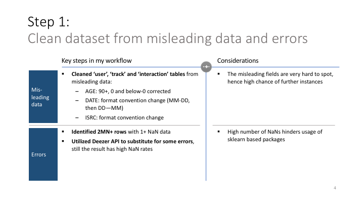
    ## 'bd', aka age of user has outliers and bias
    # Replace ages >90 years with 90 years in df_members/user age
    df_members['bd'] = df_members['bd'].apply(lambda x: x if x<=90 else 90)

    # Replace ages <0 years with np.NaN in df_members/user age
    df_members['bd'] = df_members['bd'].apply(lambda x: x if x>=0 else np.NaN)

    # Replace 0s to np.NaN in df_members/user age
    df_members['bd'].replace(0,np.NaN,inplace=True)
    
    
    
    ## Formatting date columns
    df_members['registration_init_time'] = df_members['registration_init_time'].apply(lambda x: pd.to_datetime(x, format='%Y%m%d'))
    df_members['expiration_date'] = df_members['expiration_date'].apply(lambda x: pd.to_datetime(x, format='%Y%m%d'))
    
    # Calculate the time between user registration and today (ca. 2017-Jan-31)
    df_members['days_since_registration'] = df_members['registration_init_time'].apply(lambda x: (pd.to_datetime('20170131') - x).days)

    # Calculate the time between user expiration and today (ca. 2017-Jan-31)
    df_members['days_until_expiration'] = df_members['expiration_date'].apply(lambda x: (x - pd.to_datetime('20170131')).days)
    
    
    
    # Categorize "gender" on df_members
    gender_CAT = pd.get_dummies(df_members['gender'], prefix = 'gender_CAT')
    df_members = pd.concat([df_members, gender_CAT], axis=1)
    del gender_CAT
    
    
    
    # Calculate the difference between the age of the song and the age of the user (57% NaN ratio)
    df_members['days_since_registration'] = df_members['registration_init_time'].apply(lambda x: (pd.to_datetime('20170131') - x).days)
    
    return df_members

def train_engineering(df_train):
    '''
    input: df_train
    output: df_train cleaned and engineered
    '''
    
    # Categorize "screen of listening" on df_train (1: create screen_id, 2: categorize)
    df_train['screen_id'] = df_train['source_system_tab']+'+'+df_train['source_screen_name']+'+'+df_train['source_type']
    screen_id_CAT = pd.get_dummies(df_train['screen_id'], prefix = 'screen_id_CAT')
    df_train = pd.concat([df_train, screen_id_CAT], axis=1)
    del screen_id_CAT
    
    # Count number of songs each user has listened to
    df_activity_temp = pd.DataFrame(df_train.groupby(by='msno')['song_id'].nunique()).reset_index()
    df_activity_temp.columns = ['msno','user_activity']
    df_train = df_train.merge(df_activity_temp,how='left',on='msno')
    del df_activity_temp
    
    return df_train

def merge_databases(df_train, df_members, df_full_songs):
    '''
    input: df_train, df_members, df_full_songs
    output: df_merged
    '''
    
    df_merged = (df_train.merge(df_members, on='msno', how='left')
                 .merge(df_full_songs, on='song_id', how='left')
                )
    
    return df_merged

def merged_engineering(df_merged):
    '''
    input: df_merged
    output: df_merged cleaned and engineered
    
    Notes: this function is very very heavy. To run properly on large dfs, it requires AWS and chunkified dfs
    '''    
    
    
    
    # nth time listening to this artist
    msno_group = df_merged.groupby(by='msno')
    print('*** Group by done')
    KKBOX = np.array(msno_group['artist_name_x'].nunique())
    DEEZER = np.array(msno_group['artist_name_y'].nunique())
    print('*** Uniques found')
    df_artist_freq = pd.DataFrame({'msno':np.array(list(msno_group.groups.keys())),'artist_freq':np.where(KKBOX>DEEZER,KKBOX,DEEZER)})    
    df_artist_freq.columns = ['msno','artist_freq']
    print('*** Frequencies in df')
    print('*** Merge starting')
    df_merged = df_merged.merge(df_artist_freq,how='left',on='msno')
    print('*** Merge finished')
    del df_artist_freq
    
    
    
    
    # number of genres listened
    df_merged['genre_ids'] = df_merged['genre_ids'].str.replace('|',r',')
    print('*** Replace of | to , finished')
    df_grouped = (df_merged
                  .groupby('msno',as_index=False)
                  .agg({'genre_ids':(lambda x: x.str.cat(sep=',').split(','))})
                  .rename(columns={'genre_ids':'all_genres_listened'})
                 )
    print('*** Groupby finished')
    df_grouped['number_of_genres_listened'] = df_grouped['all_genres_listened'].swifter.apply(lambda x: len(set(x)))
    print('*** Set creation finished')
    print('*** Merge starting')
    df_merged = df_merged.merge(df_grouped, on='msno',how='left')
    print('*** Merge finished')
    del df_grouped
    print('Finished number of genres listened')
    
    
    
    
    # nth time listening to this genre - apply function
    def check_genres(row):
        counter = 0
        prev_counter = 0
        for item in row['all_genres_listened']:
            multi_counter = 0
            if ',' in str(row['genre_ids']):
                for genre in row['genre_ids'].split(','):
                    if item == genre:
                        multi_counter += 1
                        if prev_counter > multi_counter:
                            multi_counter = prev_counter
                    prev_counter = multi_counter
            else:
                if item == row['genre_ids']:
                    counter += 1
        return counter if counter > multi_counter else multi_counter

    
    
    
    # nth time listening to this genre - runner
    print('*** Starting nth time this genre')
    df_merged['n_th_time_this_genre'] = df_merged.swifter.apply(check_genres,axis=1)

    
    return df_merged

3. Codifying often (re-)used functions

In this step I am defining functions that are often required and re-run in the (following) model building step. The functions are not run in the order of this notebook, but rather as-required.

3.1. Chunkifier: Read a database ‘chunkified’, i.e. in smaller pieces. This is helpful when the computation is very memory or cpu hungry

def chunk(seq, size):
    return (seq[pos:pos + size] for pos in range(0, len(seq), size))

# usage: for i, df_chunk in enumerate(chunk(df_merged_final, 100000)):

3.2. Pickle reader: For some reason pandas’ built-in pickle reader did not cope with the challenge to read some of my pickles, hence I built the below substitute function

# This unpickler was more reliable than pd.read_pickle
# filename = 'df_merged_merged_aws.pkl'

def own_read_pickle(filename):

    import pickle as pkl
    objects = []
    print(f'Pickle load of {filename} started')
    with (open(filename, 'rb')) as openfile:
        while True:
            try:
                objects.append(pkl.load(openfile))
            except EOFError:
                break

    df_output = objects[0]
    print(f'Pickle load of {filename} finished')
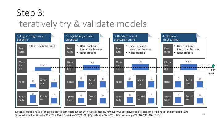
    return df_output

3.3. Model scorer: The below function provides the most important scoring metrics to evaluate model performance and returns the confusion matrix that provides the absolute figures behing these scoring metrics.

def score_model(model, X, y, gbm=False):

    # Calculate hard predictions
    if gbm:
        prediction_hard = model.predict(X,ntree_limit=model.best_ntree_limit)
    else:
        prediction_hard = model.predict(X)
    print('score_model: Predictions ready')
    
    # Score model on FBeta weighing on precision
    beta=0.3
    print(f'FBeta(b={beta}) score is: {fbeta_score(y, prediction_hard,beta)}')

    # Calculate confusion matrix
    conf_matrix = confusion_matrix(y, prediction_hard)
    TN, FP, FN, TP = conf_matrix.ravel()

    ## Scoring
    Recall = TP / (TP + FN)
    Precision=TP/(TP+FP)
    Specificity = TN / (TN + FP)
    Accuracy=(TP+TN)/(TP+TN+FP+FN)

    print('Accuracy:',Accuracy)
    print('Recall:',Recall)
    print('Precision:',Precision)
    print('Specificity:',Specificity)

    # Print confusion matrix
    return pd.DataFrame(conf_matrix, columns=
                 ['Predict (0=no relisten)', 'Predict (1=relisten)'],
                 index=['Actual (0=no relisten)', 'Actual (1=relisten)'])

4. Building the model

4.0. Create df_X by compiling ‘useful’ features and the target

This is step 0, i.e. loading the data and selecting feature-columns we (may) require. This is not to be confused with feature-selection, in this case I am loading all features that may or may not help the model.

def select_columns(df_in, target_removed=True):

    cols_not_required = ['song_id','source_system_tab','source_screen_name',
                        'source_type','gender','city','registered_via','registration_init_time',
                         'expiration_date','name','isrc','genre_ids','artist_name_x','composer',
                         'lyricist','language','track_title','album_title','artist_name_y',
                         'release_date','duration_sec','song_language_isrc','screen_id','all_genres_listened'
                        ]
    df_out = df_in.drop(cols_not_required,axis=1)
    
    if target_removed:
        df_out = df_out.drop(['target'],axis=1)
    
    return df_out

def load_dataset(filename, sample=False):
    
    df_merged = own_read_pickle(filename)
    print('load_dataset: df_merged loaded into memory')
    
    # Sample creation if needed
    if sample:
        list_of_chunks = get_user_split_data(df_merged,100000)
        df_sample = list_of_chunks[0]
        #df_sample = pd.read_pickle('df_sample_modeltraining.pkl')
        df_merged = df_sample
        print('load_dataset: sample creation done')
    
    df_X = select_columns(df_merged,target_removed=True).reset_index()
    df_X.rename({'index':'time_proxy'},axis=1,inplace=True)
    df_y = df_merged[['msno','target']]
    
    print('load_dataset: df_X,df_y created')
    
    return df_X, df_y

4.1. Checking distribution of the target

Checking the target distribution guides us whether class-imbalance measures are required. In this case the classes are balanced almost spot-on evenly.

y_train = pd.DataFrame(own_read_pickle('y_train.pkl'))
target_pcts = df_y['target'].value_counts(normalize=True) 
print(target_pcts)
target_pcts.plot(kind='bar')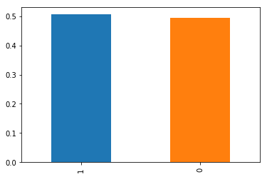

target_distribution

4.2. Decide which scoring metric to optimize on

target metrics have no imbalance
it is not crucial to catch all ‘positive’ cases, nor are we interested in negative cases
key is high precision, i.e. out of all music recommendations we want the highest number actual interesting ones, and rather recommend less but more precisely
however fully leaving recall out, would be biased
score of choice: FBeta (beta = ¹⁄₃, i.e. giving more weight to precision)

4.3. Split into train-test-validation taking user-based split

Train-test-validation split is key to tune and evaluate model performance. In our case the data is already naturally split by users (listening to overlapping songs), and keeping each user in only one of the splits seems like a logical choice. I had the guiding thought that I want to learn from the behaviour of one user and apply it to another.

Side-note: Another potential split would be based on time, i.e. I am learning from any user’s past behaviour to predict the future. However in our case the data does not have an explicit time dimension, as the re-listening targets given already give sneak peak into the future.

def get_user_split_data(df, chunksize = 100000):
    
    # list of unique users
    all_users = df['msno'].unique()
    number_of_users = all_users.shape[0]
    len_df = df.shape[0]
    chunknumbers = ceil(len_df / chunksize)
    userchunks = ceil(number_of_users/chunknumbers)
    
    df_chunks=[]
    for i in range(1,chunknumbers+1):
        print(f'Creating chunks {i} of {chunknumbers}')
        users_in_chunk = all_users[(i-1)*userchunks:i*userchunks]
        df_chunks.append(df[df['msno'].isin(users_in_chunk)])
    
    print('All chunks created')
    return df_chunks

def get_user_split_data_train_test(df_X, df_y, test_size=.2, seed=42):

    rs = np.random.RandomState(seed)
    
    total_users = df_X['msno'].unique() 
    test_users = rs.choice(total_users, 
                           size=int(total_users.shape[0] * test_size), 
                           replace=False)

    X_tr = df_X[~df_X['msno'].isin(test_users)]
    X_te = df_X[df_X['msno'].isin(test_users)]
    
    y_tr = df_y[~df_y['msno'].isin(test_users)]
    y_te = df_y[df_y['msno'].isin(test_users)]

    return X_tr, X_te, y_tr, y_te

def split_data(df_X,df_y):
    # 20% for testing and 20% for validation
    # Getting: X_train, y_train + X_val, y_val + X_test, y_test
    X_train_val, X_test, y_train_val, y_test = get_user_split_data_train_test(df_X,df_y,test_size=0.2)
    X_train, X_val, y_train, y_val = get_user_split_data_train_test(X_train_val,y_train_val,test_size=0.25)
    print('split_data: train_test split on a user base finished')

    # Dropping msno columns, which was kept for user-based splitting
    X_train = X_train.drop(['msno'],axis=1)
    y_train = y_train.drop(['msno'],axis=1)
    X_val = X_val.drop(['msno'],axis=1)
    y_val = y_val.drop(['msno'],axis=1)
    X_test = X_test.drop(['msno'],axis=1)
    y_test = y_test.drop(['msno'],axis=1)

    y_train = np.array(y_train).reshape(y_train.size,)
    y_val = np.array(y_val).reshape(y_val.size,)
    y_test = np.array(y_test).reshape(y_test.size,)
    print('split_data: msno dropped, y-s reshaped')
    
    del df_X, df_y, X_train_val, y_train_val
    
    return X_train, y_train, X_val, y_val, X_test, y_test

4.4. Preparing a baseline model

Building a baseline model is helpful to have a benchmark for later models. In the baseline model I am only using a few seemingly important features to understand how much of the target’s variance is explained when still keeping things simple.

from sklearn.linear_model import LogisticRegression
from sklearn.metrics import fbeta_score, confusion_matrix
from sklearn.preprocessing import StandardScaler

X_train_small = X_train[['user_activity','artist_freq','number_of_genres_listened','n_th_time_this_genre']].astype(float)
X_val_small = X_val[['user_activity','artist_freq','number_of_genres_listened','n_th_time_this_genre']].astype(float)

# Scale X_train to same scale
std_scale = StandardScaler()
X_train_scaled = std_scale.fit_transform(X_train_small)
X_val_scaled = std_scale.fit_transform(X_val_small)

# Apply logistic regression
lr = LogisticRegression(solver='lbfgs')
lr.fit(X_train_scaled, y_train)

score_model(lr, X_val_scaled, y_val)

FBeta(b=0.3) score is: 0.8145705294249105
Accuracy: 0.5380899961808909
Recall: 0.8510212418300653
Precision: 0.5519114101782923
Specificity: 0.1556931063744821

	Predict (0=no relisten)	Predict (1=relisten)
Actual (0=no relisten)	3119	16914
Actual (1=relisten)	3647	20833

4.5. Check pairplots if linear separation is possible

Pairplots show the relationships between all features and between each feature and the target. This latter is what we are interested in, specifically looking for separations of the target along the axis of the feature

Note: it is the bottom row of the pairplot in my case, and the linear separation by each features individual contribution is relatively low, i.e. there is no very clear groups being formed along the different values on the features x-axis

sns.pairplot((select_columns
              (df_sample,target_removed=False)
              [['user_activity','artist_freq','number_of_genres_listened','n_th_time_this_genre','target']]), 
             hue='target')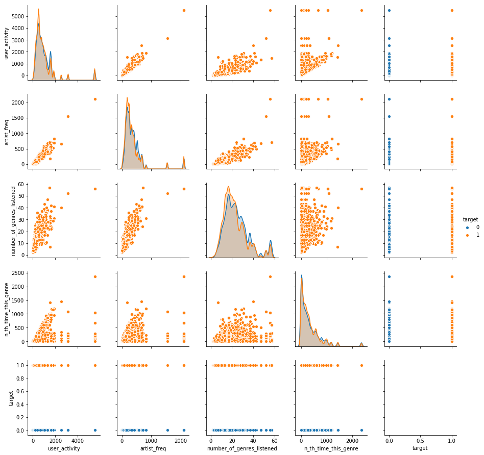

pairplot

4.6. Tree-based models

Switching to tree-based methods given low (accuracy) scores in logistic regression, clear bias towards positive predictions, and low visible separatability inferrable from the pairplots.

Random-forest classifier

from sklearn.metrics import fbeta_score, confusion_matrix
from sklearn.ensemble import RandomForestClassifier
import xgboost as xgb

# Select dataframes

X_train_small = X_train[['user_activity','artist_freq','number_of_genres_listened','n_th_time_this_genre']].astype(float)
X_val_small = X_val[['user_activity','artist_freq','number_of_genres_listened','n_th_time_this_genre']].astype(float)

# Random forest for baseline

rf = RandomForestClassifier(n_estimators = 1000, max_features = 3, min_samples_leaf = 4, n_jobs=-1)
rf.fit(X_train_small,y_train)

RandomForestClassifier(bootstrap=True, class_weight=None, criterion='gini',
            max_depth=None, max_features=3, max_leaf_nodes=None,
            min_impurity_decrease=0.0, min_impurity_split=None,
            min_samples_leaf=4, min_samples_split=2,
            min_weight_fraction_leaf=0.0, n_estimators=1000, n_jobs=-1,
            oob_score=False, random_state=None, verbose=0,
            warm_start=False)

# Random forest scoring
score_model(rf, X_val_small, y_val)

FBeta(b=0.3) score is: 0.797741149918771
Accuracy: 0.5452789072855121
Recall: 0.8297794117647059
Precision: 0.5582488251298541
Specificity: 0.19762392053112365

	Predict (0=no relisten)	Predict (1=relisten)
Actual (0=no relisten)	3959	16074
Actual (1=relisten)	4167	20313

XG Boost classifier

# Gradient boosting

gbm = xgb.XGBClassifier( 
                        n_estimators=30000,
                        max_depth=4,
                        objective='binary:logistic', #new objective
                        learning_rate=.005, 
                        subsample=.8,
                        min_child_weight=3,
                        colsample_bytree=.8,
                        n_jobs=-1
                       )

eval_set=[(X_train_small,y_train),(X_val_small,y_val)]
fit_model = gbm.fit( 
                    X_train_small, y_train, 
                    eval_set=eval_set,
                    eval_metric='error', #new evaluation metric: classification error (could also use AUC, e.g.)
                    early_stopping_rounds=50,
                    verbose=False
                   )

score_model(gbm, X_val_small, y_val)

FBeta(b=0.3) score is: 0.9040621810095893
Accuracy: 0.554849145193539
Recall: 0.9582516339869281
Precision: 0.5552057939457055
Specificity: 0.061897868516947036

	Predict (0=no relisten)	Predict (1=relisten)
Actual (0=no relisten)	1240	18793
Actual (1=relisten)	1022	23458

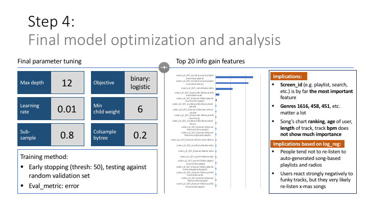
4.7. Extending the model

As the above results still can take improvements, below I am using an automatic feature selection mechanism and tweaking the hyperparameters of XG Boost (using trial-and-errors)

def tree_modelrun(X_train,y_train,X_val,y_val, xgb, select_thresh=0,select_model=None):
    
    if xgb:
        
        if select_thresh>0:
            from sklearn.feature_selection import SelectFromModel
            selection = SelectFromModel(select_model, threshold=select_thresh, prefit=True)
            X_train = selection.transform(X_train)
            X_val = selection.transform(X_val)
        
        # Gradient boosting

        model = xgb.XGBClassifier( 
                                n_estimators=30000,
                                max_depth=12,
                                objective='binary:logistic', #new objective
                                learning_rate=.01, 
                                subsample=.8,
                                min_child_weight=4,
                                colsample_bytree=.2,
                                n_jobs=-1
                               )

        eval_set=[(X_train,y_train),(X_val,y_val)]
        fit_model = model.fit( 
                            X_train, y_train, 
                            eval_set=eval_set,
                            eval_metric='error', #new evaluation metric: classification error (could also use AUC, e.g.)
                            early_stopping_rounds=50,
                            verbose=True
                           )
    else:
        # Random forest for baseline

        model = RandomForestClassifier(n_estimators = 1000, n_jobs=-1)
        model.fit(X_train,y_train)

    print(score_model(model, X_val, y_val))
    
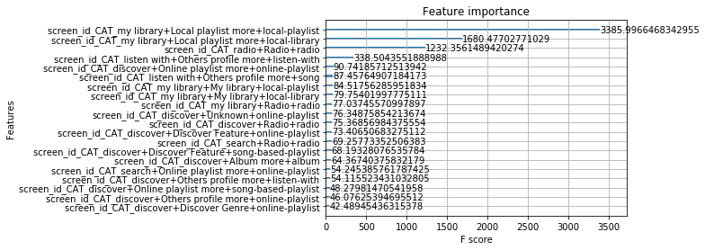
    return model

4.8. Plotting feature importance from XG Boost

def param_importance(gbm,num):
    gain = gbm.get_booster().get_score(importance_type='gain')
    return xgb.plot_importance(gbm,max_num_features=num), xgb.plot_importance(gbm, importance_type='gain',max_num_features=num), gain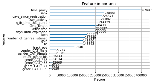

splits splits

5. – MAIN – Pulling things together

png

def feature_engineering():
    start = time.time()
    print('starting',start)

    df_train, df_members, df_full_songs = read_in_data(sample=True)
    print('Data loaded. Elapsed:',round((time.time() - start)/60,1),'minutes')

    df_merged = merge_databases(df_train, df_members, df_full_songs)
    print('df_merged created',round((time.time() - start)/60,1),'minutes')
    df_merged.to_pickle('df_merged_premod.pkl',protocol=3)
    print('df_merged premod pickled',round((time.time() - start)/60,1),'minutes')

    del df_train, df_members, df_full_songs
    print('individual dfs deleted',round((time.time() - start)/60,1),'minutes')

    df_merged = full_songs_engineering(members_engineering(train_engineering(df_merged)))

    dfs=[]
    all_chunks = get_user_split_data(df_merged,100000)
    number_of_chunks = len(all_chunks)

    for i, df_chunk in enumerate(all_chunks):
        print(f'initiating chunk number {i} of {number_of_chunks}')
        dfs.append(merged_engineering(df_chunk))
        print(f'finished chunk number {i} of {number_of_chunks} in',round((time.time() - start)/60,1),'minutes')

    with open('merged_engineered_list_preconcat.pkl', 'wb') as handle:
        pkl.dump(dfs, handle, protocol=pkl.HIGHEST_PROTOCOL)
    print(f'list pkl saved',round((time.time() - start)/60,1),'minutes')    

    print(f'concat starting at',round((time.time() - start)/60,1),'minutes')
    df_merged_postmod = pd.concat(dfs)
    print(f'concat finished at',round((time.time() - start)/60,1),'minutes')

    print(f'pickle starting at',round((time.time() - start)/60,1),'minutes')
    df_merged_postmod.to_pickle('df_merged_final_postmod.pkl',protocol=3)
    print(f'pickle finished at',round((time.time() - start)/60,1),'minutes')

    print(f'Script finished in',round((time.time() - start)/60,1),'minutes')
    print('*'*50)

def model_creation():
    start = time.time()
    start_format = time.strftime("%Y%m%d-%H%M%S")
    print(f'model_creation() started {start_format}')
    
    print('*'*25,' load_dataset initializing ','*'*10,round((time.time() - start)/60,1),'minutes')
    df_X, df_y = load_dataset('df_merged_final_postmod_aws.pkl', sample=False)
    print('*'*25,' load_dataset finished ','*'*10,round((time.time() - start)/60,1),'minutes')
    
    print('*'*25,' split_data initializing ','*'*10,round((time.time() - start)/60,1),'minutes')
    X_train, y_train, X_val, y_val, X_test, y_test = split_data(df_X,df_y)
    print('*'*25,' split_data finished ','*'*10,round((time.time() - start)/60,1),'minutes')
    del df_X, df_y
    
    X_train = X_train.astype(float)
    X_val = X_val.astype(float)
    X_test = X_test.astype(float)
    
    print('*'*25,' xgboost_modelrun initializing ','*'*10,round((time.time() - start)/60,1),'minutes')
    gbm2 = xgboost_modelrun(X_train,y_train,X_val,y_val)
    print('*'*25,' xgboost_modelrun finished ','*'*10,round((time.time() - start)/60,1),'minutes')
    
    # save the model to disk
    print('*'*25,' pickle initializing ','*'*10,round((time.time() - start)/60,1),'minutes')
    filename = time.strftime("%Y%m%d-%H%M%S") + '_xgb_aws_model.sav'
    pkl.dump(gbm2, open(filename, 'wb'))
    print('*'*25,' pickle finished ','*'*10,round((time.time() - start)/60,1),'minutes')
    print('*'*50)
    print('*'*25,' model_creation() finished ','*'*10,round((time.time() - start)/60,1),'minutes')

def final_scoring():
    start = time.time()
    start_format = time.strftime("%Y%m%d-%H%M%S")
    print(f'model_creation() started {start_format}')
    
    X_test = own_read_pickle('X_test.pkl')
    y_test = own_read_pickle('y_test.pkl')
    
    y_test = y_test[~X_test.isnull().any(axis=1)]
    X_test = X_test.dropna()
    with open('X_test_dropna.pkl', 'wb') as handle:
        pkl.dump(X_test, handle, protocol=pkl.HIGHEST_PROTOCOL)
    with open('y_test_dropna.pkl', 'wb') as handle:
        pkl.dump(y_test, handle, protocol=pkl.HIGHEST_PROTOCOL)
    
    X_train = own_read_pickle('X_train_dropna.pkl')
    y_train = own_read_pickle('y_train_dropna.pkl')

    print('*'*50,round((time.time() - start)/60,1),'minutes')
    ## 1. Logistic regression - baseline
    print('Logistic regression baseline')
    X_train_small = pd.DataFrame(X_train['screen_id_CAT_my library+Local playlist more+local-playlist'])
    X_test_small = pd.DataFrame(X_test['screen_id_CAT_my library+Local playlist more+local-playlist'])
    lr = LogisticRegression(solver='lbfgs')
    lr.fit(X_train_small, y_train)
    print(score_model(lr, X_test_small, y_test))
    filename = time.strftime("%Y%m%d-%H%M%S") + '_logbaseline_aws_model.sav'
    pkl.dump(lr, open(filename, 'wb'))
    del lr
    print(f'Saved as {filename}')

def othermodels():    
    print('*'*50,round((time.time() - start)/60,1),'minutes')
    ## 2. Logistic regression - extended
    print('Logistic regression extended')
    std_scale = StandardScaler()
    X_train_scaled = std_scale.fit_transform(X_train)
    X_test_scaled = std_scale.fit_transform(X_test)
    lr2 = LogisticRegression(solver='lbfgs')
    lr2.fit(X_train_scaled, y_train)
    print(score_model(lr2, X_test_scaled, y_test))
    filename = time.strftime("%Y%m%d-%H%M%S") + '_logextended_aws_model.sav'
    pkl.dump(lr2, open(filename, 'wb'))
    del lr2
    print(f'Saved as {filename}')
    
    print('*'*50,round((time.time() - start)/60,1),'minutes')
    ## 3. Random forest model
    print('Random forest extended')
    rf = RandomForestClassifier(n_estimators = 1000, n_jobs=-1)
    rf.fit(X_train,y_train)
    print(score_model(rf, X_test, y_test))
    filename = time.strftime("%Y%m%d-%H%M%S") + '_RF_aws_model.sav'
    pkl.dump(rf, open(filename, 'wb'))
    del rf
    print(f'Saved as {filename}')
    
    print('*'*50,round((time.time() - start)/60,1),'minutes')
    ## 4. Final xgboost model
    print('XGBoost final')
    xgb = pkl.load(open("20181029-155308_xgb_aws_model(full v4).sav", "rb"))
    print(score_model(xgb, X_test, y_test))
    print(f'Saved as 20181029-155308_xgb_aws_model(full v4).sav')

Posted on Dec 12, 2018 at 11:20

#Music #Recommendation #Logistic Regression #Random Forest #Xgboost #Kaggle #Deezer #Kkbox

Krisztian Sandor's data science blog

Using data science to solve business problems