Regression analysis of apartment prices in Budapest, Hungary
This project is about building a regression model to predict apartment prices in Budapest, Hungary based on physical, location-related and other features. This was the first standalone project I conducted in python during my bootcamp in Metis in New York - for this reason there are some natural limitations in the coding techniques.
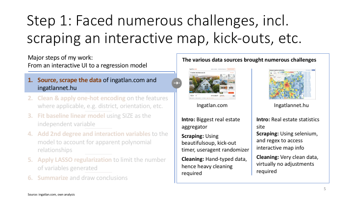
The data was scraped from ingatlan.com, a website serving arguably as the biggest real-estate selling and renting platform in Hungary.
My objective utlizing webscraping and regression models was to predict apartment selling prices in Budapest, Hungary.

0. Imports and helper functions
Below are the imports for the notebook and some helper functions utlized later in the code
Imports
# Import all necessery python packages
import pandas as pd
import numpy as np
import matplotlib.pyplot as plt
import matplotlib.dates as mdates
import re
import requests as req
from bs4 import BeautifulSoup
from urllib.parse import urljoin
from selenium import webdriver
import time
import geopy.distance
from geopy.geocoders import Nominatim
from geopy.exc import GeocoderTimedOut
import roman
import seaborn as sns
from fake_useragent import UserAgent

import patsy
import statsmodels.api as sm
import statsmodels.formula.api as smf

from sklearn.model_selection import train_test_split, KFold
from sklearn.metrics import mean_absolute_error, mean_squared_error
from sklearn.linear_model import LinearRegression, Lasso, LassoCV, RidgeCV, Ridge, lars_path
from sklearn.preprocessing import StandardScaler, PolynomialFeatures
from sklearn.pipeline import Pipeline

from IPython.display import Image

%matplotlib inline
Load list of pickled dfs and concatanate together
# Load pickle files feeded as list from the same directory
# Return all pickles concatenated into single pandas dataframe

def loadpickles(file_list):
    pickle_dfs = []

    for pickle in file_list:
        df = pd.read_pickle(pickle)
        pickle_dfs.append(df)

    df_concat = pd.concat(pickle_dfs)
    return df_concat
Calculate the distance from city centre for a given address
# Returns the distance in meters of an address
# from Vorosmarty ter (the central square of Budapest)

def distance_from_centre(address):
    if address != False:
        try:
            geolocator = Nominatim(user_agent='geopy.geocoders.options.default_user_agent')
            location_ingatlan = geolocator.geocode(address)
            #location_POI = geolocator.geocode("Vorosmarty ter, V.kerület")
            coords_ingatlan = (location_ingatlan.latitude, location_ingatlan.longitude)
            #coords_POI = (location_POI.latitude, location_POI.longitude)
            coords_POI = (47.4960918, 19.050927) # to make the code quicker, I have hard-coded the coordinates for the central square

            return(geopy.distance.vincenty(coords_ingatlan, coords_POI).meters)

        # There are lots of errors when this is running, this except tries to catch some of these errors
        except:
            return np.NaN
    else:
        return np.NaN
Check if an address exists in the Nominatim package
# Returns True if an address exists, False if does not exist

def address_exists(address):
    try:
        geolocator = Nominatim(user_agent='geopy.geocoders.options.default_user_agent')
        location_POI = geolocator.geocode(address)
        return False if location_POI is None else True
    except: #GeocoderTimedOut as e:
        return False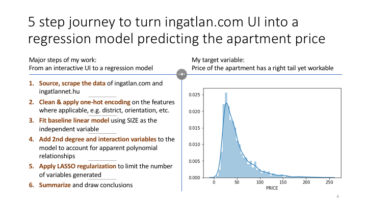
1. Scrape ingatlan.com for apartments
The below url leads to an comprehensive listing of all available apartments in Budapest. The code opens this url and takes a snapshot of each apartment’s summary page (i.e. the page with the search results), then opens each apartment’s detailed page (i.e. where all details for a single apartment is available) and downloads all seemingly important information.
Initiate run
# Initial search url to be scraped (filter: all appartments in Budapest, Hungary)
url = 'https://ingatlan.com/szukites/elado+lakas+budapest'

# starting from 1st apartment on the url and downloading data for all
df_import = ingatlan_todataframe(url, 1, 1)
df_import.to_pickle('all_pages_ingatlan.pkl')
Scrape url as (beautiful-)soup object run parser
def ingatlan_todataframe(url, starting_page, run_count):

    # Creates fake header and useragent for scraping
    ua = UserAgent()
    header = {
        'User-Agent': ua.random
    }

    # Ingatlan.com accepts max of 20 real estate listings per page
    max_listing_per_page = 20
    page_str = '?page='

    # Scrapes listing page=1 with 20 listings to start with
    r_ingatlan = req.get(url, headers=header)
    soup = BeautifulSoup(r_ingatlan.content,"lxml")

    # Takes the counter from the listing page showing the number of total results of search url
    listing_count = int(soup.find('div', {'class':'results__number'}).attrs['data-listings-count'].replace(' ',''))

    # Initiates list of dfs' and df_backups' containing df of the results from each individual listing page
    dfs = []
    df_backups = []

    # Loops thru each page of the search results
    for page_num in range(starting_page,(listing_count // max_listing_per_page)+1):

        # Creates fake header and useragent for scraping
        ua = UserAgent()
        header = {
            'User-Agent': ua.random
        }

        # Compiles each page's url and opens, scrapes using beautifulsoup
        listing_url_page = urljoin(url,page_str) + str(page_num)
        print('Scraping:',listing_url_page)
        r_ingatlan = req.get(listing_url_page, headers=header)
        soup = BeautifulSoup(r_ingatlan.content,"lxml")

        # Collects all information to be found on each page of the search results and appends to dfs list
        dfs.append(ingatlan_parser(soup,run_count,page_num)) # <-- runs the below parser function

        # Save backup per each 50 pages and save to pickle: backup_[pagenum].pkl
        if page_num % 10 == 0:
            #break #remove for full run, otherwise only running page=1
            df_backups = dfs.copy()
            df_backup = pd.concat(df_backups)
            path = 'backup_' + str(page_num) + '.pkl'
            df_backup.to_pickle(path)
            print('Saved backup:', path)
            del df_backup
            del df_backups
            del path

    # Once all pages have been scraped concatenates all individual page dfs into a single df and returns df as result
    df_import = pd.concat(dfs)

    return(df_import)
Put the scraped soup object into dataframe (run within above function)
# Gets soup object from real estate listing page and scrape all infos from there and detailed pages
# Returns df of all real estates on listing page
def ingatlan_parser(soup, run_count, where_am_i):
dfs = []
urls = []
i = 1
error = False
# Check if error handler has rerun the code already or this is the first run
# Scrape all available infos from the real estate list page info-card
#for div in soup.find_all('div', {'class':'listing js-listing '}):
listings = soup.find_all('div', class_='listing js-listing ')
for div in listings:
# Initiate feature variables, left as NaN for those not existent on detailed real estate page
ingatlan_id = np.NaN
ingatlan_size = np.NaN
ingatlan_price = np.NaN
ingatlan_rooms = np.NaN
ingatlan_floor = np.NaN
ingatlan_address_withdistrict = np.NaN
ingatlan_quality = np.NaN
ingatlan_yearbuilt = np.NaN
ingatlan_floorsinbuilding = np.NaN
ingatlan_lift = np.NaN
ingatlan_orientation = np.NaN
ingatlan_view = np.NaN
ingatlan_metro = np.NaN
# Error handling: poorly entered data causes errors, in this case return np.NaN values
try:
# Read address from listing page
address = div.find('div', {'class':'listing__address'}).text
ingatlan_address_withdistrict = False if address_exists(address) == False else address
ingatlan_id = div.attrs['data-id']
# Navigate to detailed info of the real estate
BASE_URL = 'https://ingatlan.com/'
url_ingatlan = urljoin(BASE_URL, ingatlan_id)
# Print listing page url being scraped
#print('Scraping:',url_ingatlan)
# Creates fake header and useragent for scraping
ua = UserAgent()
header = {
'User-Agent': ua.random
}
# Call listing page and pull html into soup_ingatlan 'beautifulsoup' object
r_ingatlan = req.get(url_ingatlan, headers=header)
soup_ingatlan = BeautifulSoup(r_ingatlan.content,"lxml")
# Read all required info from real estate detailed page (those without IDs)
# Loop thru each table with feature data (has no IDs)
for table in (soup_ingatlan
.find('div', {'class':'card details'})
.find('div', {'class':'paramterers'})
.find_all('table')
):
# Loop thru cells of each table
for td in table.find_all('td'):
# Once flag is reached fill-in flag
if td.text == 'Ingatlan állapota':
ingatlan_quality = td.findNextSibling().text
if td.text == 'Építés éve':
ingatlan_yearbuilt = td.findNextSibling().text
if td.text == 'Emelet':
ingatlan_floor = td.findNextSibling().text
if td.text == 'Épület szintjei':
ingatlan_floorsinbuilding = td.findNextSibling().text
if td.text == 'Lift':
ingatlan_lift = td.findNextSibling().text
if td.text == 'Tájolás':
ingatlan_orientation = td.findNextSibling().text
if td.text == 'Kilátás':
ingatlan_view = td.findNextSibling().text
#Find which public transport is nearby the real estate (if any)
ingatlan_metro = True if (soup_ingatlan.find('a', class_='subway')) is not None else False
# If address was not in title, do second try to extract from 'long description'
if ingatlan_address_withdistrict == False:
long_decription = soup_ingatlan.find('div', {'class':'long-description'}).text.strip()
ingatlan_address_withdistrict = re.search(r'\w*\s*[uU]tca', long_decription)
if ingatlan_address_withdistrict is not None:
try:
ingatlan_address_withdistrict = ingatlan_address_withdistrict.group()[0]
except:
ingatlan_address_withdistrict = False
else:
ingatlan_address_withdistrict = False
# Read all required info from real estate detailed page (those with IDs)
#ingatlan_id = soup_ingatlan.find('b', {'class':'listing-id'}).text #.split()[1] # Decomissioned - not useful
ingatlan_size = soup_ingatlan.find('div', {'class':'parameter parameter-area-size'}).find('span', {'class':'parameter-value'}).text
ingatlan_price = soup_ingatlan.find('div', {'class':'parameter parameter-price'}).find('span', {'class':'parameter-value'}).text
ingatlan_rooms = soup_ingatlan.find('div', {'class':'parameter parameter-room'}).find('span', {'class':'parameter-value'}).text
ingatlan_newlybuilt = soup_ingatlan.find('span', {'class':'label label--newly-built'})
#ingatlan_district = soup_ingatlan.find('div', {'id':'map-nav-links'}).find_all('a')[1].text
#ingatlan_address = soup_ingatlan.find('a', {'class':'map-link is-map-link-active'}).text #decommissioned due to speed limitations
# If poor data source quality return np.NaN for the appartment values
except:
pass
error = True
# Create numpy array from all the avaiable infos on the real estate
appartment = np.array([
ingatlan_id,
ingatlan_size,
ingatlan_price,
ingatlan_rooms,
ingatlan_floor,
ingatlan_address_withdistrict,
distance_from_centre(ingatlan_address_withdistrict), # + ' ' + ingatlan_district),
ingatlan_quality,
ingatlan_yearbuilt,
ingatlan_floorsinbuilding,
ingatlan_lift,
ingatlan_orientation,
ingatlan_view,
ingatlan_metro
])
# Reshape array to fit pandas structure
appartment = appartment.reshape(1,appartment.size)
# Create pandas df from real estate numpy array
df_appartment = pd.DataFrame(appartment, columns = [
'ID',
'SIZE',
'PRICE',
'ROOMS',
'FLOOR',
'ADDRESS',
'DISTANCE_FROM_CENTRE',
'QUALITY',
'YEAR_BUILT',
'FLOORS_IN_BUILDING',
'LIFT',
'ORIENTATION',
'VIEW',
'METRO_NEARBY'
])
# Append real estate df to list with all previous dfs
dfs.append(df_appartment)
#break #remove for full run
if error == True:
#print('Error avoided at:\n', appartment)
error = False
#i += 1
#if (i % 10 == 0):
#print('Waiting 2 seconds...')
#time.sleep(2)
#print('Continuing...')
# Try to concat together all dfs in appended list - sometimes failes due to unclear reasons in this case retry once
try:
df = pd.concat(dfs)
run_count = 1
df.set_index('ID',inplace=True)
return df
# Re-run 5 times to try again, after that raise error and tell which df caused the error
except:
if run_count < 6:
re_starting_page = where_am_i - ((where_am_i % 10) if where_am_i % 10 != 0 else 10) + 1
print('Re-running starting from:', re_starting_page)
ingatlan_todataframe(url, re_starting_page, run_count + 1)
else:
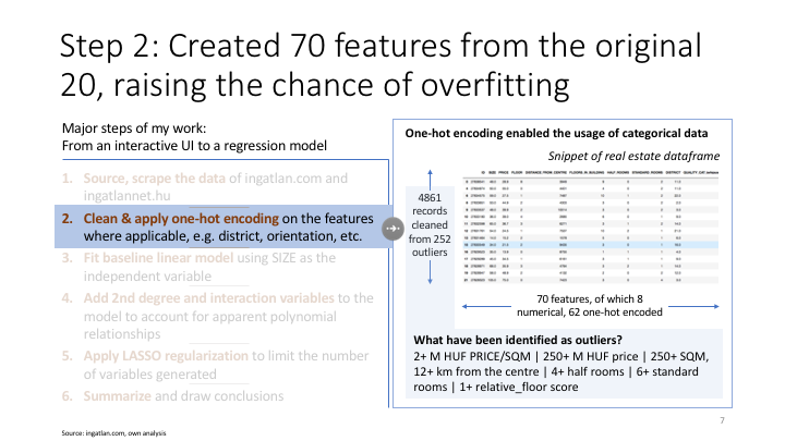
raise ValueError('Cannot concatenate this df:', dfs)2. Clean the scraped data
Below I am cleaning the data and also creating meaningful column names later to be used a regression features
# Cleans dataframe collected from ingatlan.com to be ready for regression analysis

df = df_import.copy()

# Once apartment data is saved (e.g. partial data to be extended) the below can import it and append together
#df = loadpickles(['backup_1-30.pkl','backup_31-70.pkl','backup_71-100.pkl','backup_101-170.pkl','backup_171-190.pkl','backup_191-250.pkl','backup_251-270.pkl','backup_271-330.pkl'])
#df = loadpickles(['backup_101-170.pkl','backup_171-190.pkl','backup_191-250.pkl','backup_251-270.pkl','backup_271-330.pkl','backup_331-340.pkl','backup_341-380.pkl','backup_381-400.pkl','backup_401-470.pkl','backup_471-490.pkl','backup_491-510.pkl','backup_511-520.pkl','backup_521-530.pkl','backup_531-580.pkl','backup_581-600.pkl','backup_601-610.pkl','backup_611-630.pkl','backup_671-690.pkl','backup_691-730.pkl','backup_741-860.pkl','backup_871-910.pkl','backup_911-930.pkl','backup_931-940.pkl','backup_941-960.pkl','backup_961-1090.pkl'])

# Cleaning out df
df.reset_index(inplace=True)
df.drop_duplicates(['ID'], inplace=True)

# Makings sure NaN everywhere with missing data
#df.loc[df['FLOORS_IN_BUILDING'] == 'nincs megadva','FLOORS_IN_BUILDING'] = np.NaN
df.loc[df['FLOOR'] == 'nincs megadva','FLOOR'] = np.NaN
df.loc[df['ORIENTATION'] == 'nincs megadva','ORIENTATION'] = np.nan
df.loc[df['VIEW'] == 'nincs megadva','VIEW'] = np.nan
df.loc[df['QUALITY'] == 'nincs megadva','QUALITY'] = np.nan
df.loc[df['LIFT'] == 'nincs megadva','LIFT'] = np.nan

# Parsing that has to happen before np.NaN assignment
df = df.loc[~df['FLOORS_IN_BUILDING'].str.contains('nincs megadva')] #delete no floor buildings
df.loc[df['ROOMS'].str.contains('fél'), 'HALF_ROOMS'] = df['ROOMS'].str.split('+',1).str[1].str.replace('[^\d.]*', '')
df.loc[~df['ROOMS'].str.contains('fél'), 'HALF_ROOMS'] = 0
df.loc[df['ROOMS'].str.contains('fél'), 'STANDARD_ROOMS'] = df['ROOMS'].str.split('+',1).str[0]
df.loc[~df['ROOMS'].str.contains('fél'), 'STANDARD_ROOMS'] = df['ROOMS']

# Formatting district from roman into arabic numbers
df['DISTRICT'] = df['ADDRESS'].str.split(',',1).str[1].str.split('.',1).str[0].str.strip().apply(lambda x: int(roman.fromRoman(x)) if isinstance(x, str) else np.NaN)

# One-Hot categorization
QUALITY_CAT = pd.get_dummies(df['QUALITY'], prefix = 'QUALITY_CAT')
YEAR_BUILT_CAT = pd.get_dummies(df['YEAR_BUILT'], prefix = 'YEAR_BUILT_CAT')
LIFT_CAT = pd.get_dummies(df['LIFT'], prefix = 'LIFT_CAT')
ORIENTATION_CAT = pd.get_dummies(df['ORIENTATION'], prefix = 'ORIENTATION_CAT')
VIEW_CAT = pd.get_dummies(df['VIEW'], prefix = 'VIEW_CAT')
METRO_NEARBY_CAT = pd.get_dummies(df['METRO_NEARBY'], prefix='METRO_NEARBY_CAT')
DISTRICT_CAT = pd.get_dummies(df['DISTRICT'], prefix='DISTRICT_CAT')

# Concatenate original df with categorization columns
df = pd.concat([df, QUALITY_CAT, YEAR_BUILT_CAT, LIFT_CAT, ORIENTATION_CAT, VIEW_CAT, METRO_NEARBY_CAT, DISTRICT_CAT], axis=1)

# Further cleaning of string data into int
df['FLOORS_IN_BUILDING'] = df['FLOORS_IN_BUILDING'].replace({'földszintes':1, 'több mint 10':11})

# Replacing string nan with np.Nan and removing nan related category columns
df.replace('nan',np.NaN,inplace=True)
df.drop(df.filter(regex='nan').columns, inplace=True, axis=1)

# Parse and transform the dataframe
df['SIZE'] = df['SIZE'].str.replace(',', '.').str.replace('[^\d.]*', '').astype(float)
df['PRICE'] = df['PRICE'].str.replace(',', '.').str.replace('[^\d.]*', '').astype(float)
df['PRICE_PER_SQM'] = (df['PRICE'] / df['SIZE']) * 1000
df['STREET'] = df['ADDRESS'].str.split(',',1).str[0]
df['FLOOR'] = df['FLOOR'].replace({'földszint':0, 'szuterén':0, 'félemelet':1, '10 felett':11})

# Deletes non-numeric columns, all should be categorized above
del df['ROOMS']
del df['ADDRESS']
#del df['QUALITY']
del df['YEAR_BUILT']
del df['LIFT']
del df['ORIENTATION']
del df['VIEW']
del df['METRO_NEARBY']
del df['STREET']
#del df['DISTRICT']

# Replacing NaNs
df = df.replace(-1, np.nan)
df.dropna(inplace=True)

# Make all values numeric (if possible, leave non-numeric as-is)
df = df.apply(pd.to_numeric, errors='ignore')

# Adding indicator for how high the appartment is within the building
df['RELATIVE_FLOOR'] = df['FLOOR'] / df['FLOORS_IN_BUILDING']

# Rounding distance from centre to int
df['DISTANCE_FROM_CENTRE'] = df['DISTANCE_FROM_CENTRE'].round().astype(int)
df['PRICE_PER_SQM'] = df['PRICE_PER_SQM'].round().astype(int)

df.head(15)
3. Scrape ingatlannet.hu for district real estate price indices
As an additional source of information I am using ingatlannet.hu to access district-by-district real estate price indices to be utilized as a feature in the regression model
# Scrape past district level house price statistics

dfs_priceindex = []
# Fake user agent for scraping
ua = UserAgent()
header = {'User-Agent': ua.random}

# URL of ingatlannet price statistics per district in Budapest
url_pricestats = 'https://www.ingatlannet.hu/statisztika/Budapest'

# Call listing page and pull html into soup_ingatlan 'beautifulsoup' object
r_pricestats = req.get(url_pricestats, headers=header)
soup_price = BeautifulSoup(r_pricestats.content,"lxml")

# List the container with the district links
district_container = (soup_price
                 .find('div', {'class':'telepulesLista bgwhite col-sm-3 col-xs-12'})
                 .find_all('li',{'class':'col-sm-12 col-xs-6 col-xxs-12'})
                )

# Loop thru district container
for district_list in district_container:

    # Extract district names (into int) and href links
    district_longname = district_list.find('a').text
    district_romannum = district_longname.split(',')[1].strip().split('.')[0]
    district_num = int(roman.fromRoman(district_romannum))

    district_subpage_tobeformatted = district_list.find('a').attrs['href']
    district_subpage_readyforbrowser = district_subpage_tobeformatted.replace(' ','%20')
    district_html = urljoin('https://www.ingatlannet.hu/',district_subpage_readyforbrowser)

    # Open district subpage
    header = {'User-Agent': ua.random}
    r_district = req.get(district_html, headers=header)
    soup_district = BeautifulSoup(r_district.content,"lxml")

    # Extract district price data
    district_pricelist = (soup_district
                          .find('div',{'class','col-xs-12 margin-sm-vertical hidden-xs'})
                          .find_all('a')[1]
                         )

    historic_price_list = re.findall(r'\d\d\d\d-\d\d","avg":(\d*)',str(district_pricelist)) #"avg":309943

    # Calculate yoy index
    try:
        price_now = int(historic_price_list[-1])
        price_yearago = int(historic_price_list[-13])
        yoy_percentage = (price_now-price_yearago)/price_yearago * 100

        # Create numpy array from all the avaiable infos on the real estate
        district_priceindex = np.array([district_num,
                                        yoy_percentage,
                                        price_now])

        # Reshape array to fit pandas structure
        district_priceindex = district_priceindex.reshape(1,district_priceindex.size)

        # Create pandas df from real estate numpy array
        df_district_priceindex = pd.DataFrame(district_priceindex, columns = [
            'DISTRICT_NUM',
            'YOY_PERCENTAGE',
            'AVG_PRICE'
        ])

        # Append real estate df to list with all previous dfs
        dfs_priceindex.append(df_district_priceindex)
    except:
        print('Error',district_priceindex)

# Summarize final data
df_priceindex = pd.concat(dfs_priceindex)
#df_priceindex.to_pickle('price_index2.pkl')
#df_priceindex = pd.read_pickle('price_index2.pkl')
# Merging downloaded price indices with the ingatlan.com data
df_merged = df.merge(df_priceindex, left_on = 'DISTRICT', right_on = 'DISTRICT_NUM', how='left')
del df_merged['DISTRICT_NUM']
df = df_merged.copy()4. Observing the data
Best is to examine all of it in detail however, in my case the dataset is very large. Hence I am extracting aggregated information (what is data type, how many entries are there, etc.) and examine a random subset in detail. Make sure the data is clean (remove NaN, for example) and meaningful (e.g., if the number of customers is negative, there is a problem)
pd.set_option("display.max_columns",df.columns.nunique())
df.describe()
# Building smaller_df to check in pairplot
smaller_df= df.loc[:,['SIZE','FLOOR','DISTANCE_FROM_CENTRE','FLOORS_IN_BUILDING',
'HALF_ROOMS','STANDARD_ROOMS','PRICE_PER_SQM','YOY_PERCENTAGE','AVG_PRICE','RELATIVE_FLOOR','PRICE']]sns.pairplot(smaller_df) Key observations
- (from .info) all columns are all numeric and all nan-s are dropped
- ID does not make sense as a feature variable
- PRICE has a really long tail
- SIZE MAX seems unreasonable (1100 SQM?)
- DISTANCE_FROM_CENTRE MAX and MEAN seems unreasonable (max:1257km and mean: 44km)
- HALF_ROOMS MAX seems unreasonable (10 half rooms?)
- STANDARD ROOMS MAX seems unreasonable (24 rooms?)
- FLOOR and FLOORS_IN_BUILDING seem to be very correlated
- SIZE and STANDARD_ROOMS seem to be very correlated as well
- RELATIVE_FLOOR should be max 1
Based on the above observations I am dropping some outliers (note: droppings surely have overlaps, and to make it nicer it would good to check these first).
Dropping outliers
starting_observations = df.ID.nunique()

print('Starting number of observations:', df.ID.nunique())
print('Dropping:',df[df['PRICE_PER_SQM'] >= 2000].ID.nunique(), 'appartments that have 2+ M HUF PRICE/SQM')
print('Dropping:',df[df['PRICE'] >= 250].ID.nunique(), 'appartments that cost 250+ M HUF')
print('Dropping:',df[df['SIZE'] >= 200].ID.nunique(), 'appartments that are 250+ SQM')
print('Dropping:',df[df['DISTANCE_FROM_CENTRE'] >= 12000].ID.nunique(), 'appartments that 12+ km from the centre')
print('Dropping:',df[df['HALF_ROOMS'] >= 4].ID.nunique(), 'appartments with 4+ half rooms')
print('Dropping:',df[df['STANDARD_ROOMS'] >= 6].ID.nunique(), 'appartments with 6+ standard rooms')
print('Dropping:',df[df['RELATIVE_FLOOR'] > 1].ID.nunique(), 'appartments with 1+ realtive_floor score')

df = df[df['PRICE_PER_SQM'] < 2000]
df = df[df['PRICE'] < 250]
df = df[df['SIZE'] < 200]
df = df[df['DISTANCE_FROM_CENTRE'] < 12000]
df = df[df['HALF_ROOMS'] < 4]
df = df[df['STANDARD_ROOMS'] < 6]
df = df[df['RELATIVE_FLOOR'] <= 1]

df.dropna(inplace=True)

print('Dropped', starting_observations - df.ID.nunique(), 'number of records. We are left with',df.ID.nunique(),'records')smaller_df= df.loc[:,['SIZE','FLOOR','DISTANCE_FROM_CENTRE','FLOORS_IN_BUILDING',
'HALF_ROOMS','STANDARD_ROOMS','PRICE_PER_SQM','YOY_PERCENTAGE','AVG_PRICE','RELATIVE_FLOOR','PRICE']]
sns.pairplot(smaller_df) 5. Extracting the descriptive statistics
Correlation matrix, seaborn plots (to check for colinearity; compare what you see with human intuition) and probability distributions. Linear regression will be useful if the target variable has a fairly symmetric distribution (e.g., it might look close to a normal distribution). Look at the error vs. y_pred plot for any weirdness (for example, due to bimodal distribution).
smaller_df.corr()Key Observations:
- FLOOR and RELATIVE FLOOR very correlated
- SIZE and STANDARD_ROOMS seem to be very correlated as well
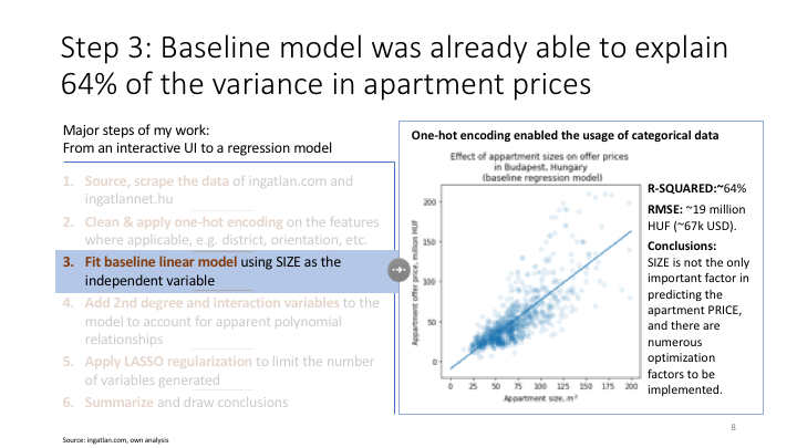
6. Building a baseline model
Using only one feature to see the fit immediately and understand how a regression model is performing on my target data. This model is not intended for ‘production’, it is rather a test and setup step in the process
Train-test split
# Assign features and target variables (using SIZE to predict PRICE_LOG)
X, y = df.drop(['ID','PRICE','PRICE_LOG','PRICE_PER_SQM'],axis=1), df['PRICE']
X_train, X_test, y_train, y_test = train_test_split(X, y, test_size=0.3)
Linear regression model (using sklearn)
# Build up baseline model with only size variable
selected_columns_1 = ['SIZE']
lr_baseline = LinearRegression()
lr_baseline.fit(X_train.loc[:,selected_columns_1],y_train)
lr_baseline.coef_, lr_baseline.intercept_
Evaluate model performance
# Performance on training data
plt.scatter(X_train['SIZE'],y_train,alpha=.1)
vec1 = np.linspace(0,200,6)
plt.plot(vec1, lr_baseline.intercept_ + lr_baseline.coef_[0]*vec1)
### Performance on test data
plt.scatter(X_test['SIZE'],y_test,alpha=.1)
vec1 = np.linspace(0,200,6)
plt.plot(vec1, lr_baseline.intercept_ + lr_baseline.coef_[0]*vec1)
plt.title(r"Effect of appartment sizes on offer prices " "\n" r" in Budapest, Hungary " "\n" r" (baseline regression model)")
plt.xlabel(r'Appartment size, $m^2$')
plt.ylabel(r'Appartment offer price, million HUF')# Get the predictions on the test set
test_set_pred1 = lr_baseline.predict(X_test.loc[:,selected_columns_1])# Plot predicted vs actual
plt.scatter(test_set_pred1,y_test,alpha=.1)
plt.plot(np.linspace(0,140,1000),np.linspace(0,130,1000))## Residual Plot
## Plot predicted vs actual
plt.scatter(y_test,y_test-test_set_pred1,alpha=.1)
plt.plot(np.linspace(0,150,1000),np.linspace(0,0,1000))np.sqrt(mean_squared_error(y_test, test_set_pred1)), mean_absolute_error(y_test,test_set_pred1)print('Baseline regression test R^2:', lr_baseline.score(X_test.loc[:,selected_columns_1], y_test))7. Building an expanded model
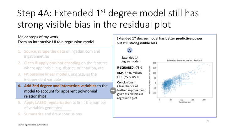
The next model is a expanded versus the baseline model, however it still is not meant for ‘production’. It is run with a few features, so it is still humanly interpretable. Plot distribution of target variable, errors vs. predicted value to see if non-linearity or heteroskedasticity are an issue. Check fit of the model.
Linear regression model (using sklearn)
# Build up expanded model
selected_columns_2 = ['SIZE','FLOOR','DISTANCE_FROM_CENTRE','YOY_PERCENTAGE','AVG_PRICE']
lr_expanded = LinearRegression()
lr_expanded.fit(X_train.loc[:,selected_columns_2],y_train)
print('Intercept:',lr_expanded.intercept_)
print(list(zip(selected_columns_2,lr_expanded.coef_)))
Evaluate model performance
# Get the predictions on the test set
test_set_pred2 = lr_expanded.predict(X_test.loc[:,selected_columns_2])
# Plot predicted vs actual
plt.scatter(test_set_pred2,y_test,alpha=.1)
plt.plot(np.linspace(0,120,1000),np.linspace(5,100,1000))## Residual Plot
## Plot predicted vs actual
plt.scatter(y_test,y_test-test_set_pred2,alpha=.1)
plt.plot(np.linspace(0,150,1000),np.linspace(0,0,1000))np.sqrt(mean_squared_error(y_test, test_set_pred2)), mean_absolute_error(y_test,test_set_pred2)print('Expanded regression test R^2:', lr_expanded.score(X_test.loc[:,selected_columns_2], y_test))Check statsmodels summary output
# Create your model
model = sm.OLS(y_train,sm.add_constant(X_train.loc[:,selected_columns_2]))
# Fit your model to your training set
fit = model.fit()
# Print summary statistics of the model's performance
fit.summary()
8. Build a complete model
Run with all features and run key diagnostics. Do you need all of the features or can you discard some of them? Are the coefficients (betas) statistically significant?
Linear regression model (using sklearn)
# Build up complete model
lr_complete = LinearRegression()
lr_complete.fit(X_train,y_train)
#print('Intercept:',lr_complete.intercept_)
#list(zip(X.columns,lr_complete.coef_))
Evaluate model performance
# Get the predictions on the test set
test_set_pred3 = lr_complete.predict(X_test)
# Plot predicted vs actual
plt.scatter(test_set_pred3,y_test,alpha=.1)
plt.plot(np.linspace(0,125,1000),np.linspace(10,125,1000))## Residual Plot
## Plot predicted vs actual
plt.scatter(y_test,y_test-test_set_pred3,alpha=.1)
plt.plot(np.linspace(0,150,1000),np.linspace(0,0,1000))np.sqrt(mean_squared_error(y_test, test_set_pred3)), mean_absolute_error(y_test,test_set_pred3)print('Complete regression test R^2:', lr_complete.score(X_test, y_test))# Create your model
model = sm.OLS(y_train,sm.add_constant(X_train))
# Fit your model to your training set
fit = model.fit()
# Print summary statistics of the model's performance
fit.summary()Refine model (based on above validation results)
# Reduction of number of features based on above P(t) values
df['Quality_CAT_befejezetlen-felujitott'] = (np.array(df['QUALITY_CAT_befejezetlen'])
                                             + np.array(df['QUALITY_CAT_felújított']))
df['YEAR_BUILT_CAT_before2000'] = (np.array(df['YEAR_BUILT_CAT_1950 előtt'])
                                   + np.array(df['YEAR_BUILT_CAT_1950-1980 között'])
                                   + np.array(df['YEAR_BUILT_CAT_1981-2000 között']))
df['YEAR_BUILT_CAT_2001-2014'] = (np.array(df['YEAR_BUILT_CAT_2001-2010 között'])
                                   + np.array(df['YEAR_BUILT_CAT_2011'])
                                   + np.array(df['YEAR_BUILT_CAT_2012'])
                                   + np.array(df['YEAR_BUILT_CAT_2013'])
                                   + np.array(df['YEAR_BUILT_CAT_2014']))
df['ORIENTATION_CAT_D-DK-DNY'] = (np.array(df['ORIENTATION_CAT_dél'])
                                   + np.array(df['ORIENTATION_CAT_délkelet'])
                                   + np.array(df['ORIENTATION_CAT_délnyugat']))
df['ORIENTATION_CAT_E-EK-ENY'] = (np.array(df['ORIENTATION_CAT_észak'])
                                   + np.array(df['ORIENTATION_CAT_északkelet'])
                                   + np.array(df['ORIENTATION_CAT_északnyugat']))
# Reduction of number of features based on above P(t) values
X_iter2, y_iter2 = df.drop(['ID','PRICE','PRICE_LOG','PRICE_PER_SQM',
'QUALITY_CAT_befejezetlen','QUALITY_CAT_felújított','YEAR_BUILT_CAT_1950 előtt','YEAR_BUILT_CAT_1950-1980 között',
'YEAR_BUILT_CAT_1981-2000 között','YEAR_BUILT_CAT_2001-2010 között','YEAR_BUILT_CAT_2011','YEAR_BUILT_CAT_2012',
'YEAR_BUILT_CAT_2013','YEAR_BUILT_CAT_2014','ORIENTATION_CAT_dél','ORIENTATION_CAT_délkelet','ORIENTATION_CAT_délnyugat',
'ORIENTATION_CAT_észak','ORIENTATION_CAT_északkelet','ORIENTATION_CAT_északnyugat',
'LIFT_CAT_nincs','DISTRICT','YEAR_BUILT_CAT_2020'
],axis=1), df['PRICE']
X_train_iter2, X_test_iter2, y_train_iter2, y_test_iter2 = train_test_split(X_iter2, y_iter2, test_size=0.3,random_state=42)Build refined model
# Create your model
model = sm.OLS(y_train_iter2,sm.add_constant(X_train_iter2))
# Fit your model to your training set
fit = model.fit()
# Print summary statistics of the model's performance
fit.summary()
# Build up complete model
lr_complete_iter2 = LinearRegression()
lr_complete_iter2.fit(X_train_iter2,y_train_iter2)
#print('Intercept:',lr_complete.intercept_)
#list(zip(X.columns,lr_complete.coef_))Evaluate refined model
# Get the predictions on the test set
test_set_pred4 = lr_complete_iter2.predict(X_test_iter2)
# Plot predicted vs actual
plt.scatter(test_set_pred4,y_test_iter2,alpha=.1)
plt.plot(np.linspace(0,125,1000),np.linspace(10,100,1000))## Residual Plot
## Plot predicted vs actual
plt.scatter(y_test_iter2,y_test_iter2-test_set_pred4,alpha=.1)
plt.plot(np.linspace(0,150,1000),np.linspace(0,0,1000))np.sqrt(mean_squared_error(y_test_iter2, test_set_pred4)), mean_absolute_error(y_test_iter2,test_set_pred4)print('Complete regression test R^2:', lr_complete_iter2.score(X_test_iter2, y_test_iter2))9. Apply regularization
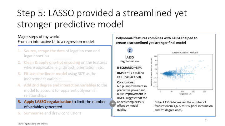
By applying regularization on the features the variance explained by the model can be improved. Below I am testing both Ridge and Lasso regularization, where ridge reduces (but not eliminating) the coefficients of the less relevant features and Lasso eliminating unnecessary features.
X, y = df.drop(['ID','PRICE','PRICE_LOG','PRICE_PER_SQM',
                            'QUALITY_CAT_befejezetlen','QUALITY_CAT_felújított','YEAR_BUILT_CAT_1950 előtt','YEAR_BUILT_CAT_1950-1980 között',
                            'YEAR_BUILT_CAT_1981-2000 között','YEAR_BUILT_CAT_2001-2010 között','YEAR_BUILT_CAT_2011','YEAR_BUILT_CAT_2012',
                            'YEAR_BUILT_CAT_2013','YEAR_BUILT_CAT_2014','ORIENTATION_CAT_dél','ORIENTATION_CAT_délkelet','ORIENTATION_CAT_délnyugat',
                            'ORIENTATION_CAT_észak','ORIENTATION_CAT_északkelet','ORIENTATION_CAT_északnyugat',
                            'LIFT_CAT_nincs','DISTRICT','YEAR_BUILT_CAT_2020'
               ],axis=1), df['PRICE']

# Hold out 20% of the data for final testing and 20% for validation
X_train_val, X_test, y_train_val, y_test = train_test_split(X, y, test_size=0.2)
X_train, X_val, y_train, y_val = train_test_split(X_train_val, y_train_val, test_size=.25)

# Applying scaler
scaler = StandardScaler()
X_train_scaled = scaler.fit_transform(X_train)
X_test_scaled = scaler.transform(X_test)
No regularization (for baseline)
lr_model_linear = LinearRegression()
lr_model_linear.fit(X_train,y_train)
test_set_pred_linear = lr_model_linear.predict(X_test)
np.sqrt(mean_squared_error(y_test, test_set_pred_linear)), mean_absolute_error(y_test,test_set_pred_linear)
print('LINEAR regression test R^2:', lr_model_linear.score(X_test, y_test))LASSO (manual alpha)
## Finding the "best" value of lambda (alpha) with a single train/valid split
alphalist = 10**(np.linspace(-3,4,200))
err_vec_val = np.zeros(len(alphalist))
err_vec_train = np.zeros(len(alphalist))

for i,curr_alpha in enumerate(alphalist):

    steps = [('standardize', StandardScaler()), ('lasso', Lasso(alpha = curr_alpha))]

    pipe = Pipeline(steps)
    pipe.fit(X_train, y_train)
    val_set_pred_lasso = pipe.predict(X_val)
    err_vec_val[i] = np.sqrt(np.mean((val_set_pred_lasso - y_val)**2))

    train_set_pred_lasso = pipe.predict(X_train)
    err_vec_train[i] = np.sqrt(np.mean((train_set_pred_lasso - y_train)**2))

## This is the minimum error achieved on the validation set
## across the different alpha values we tried

np.min(err_vec_val)
# plot the curves of both the training error and test error as alpha changes
plt.plot(np.log10(alphalist),err_vec_val)
plt.plot(np.log10(alphalist),err_vec_train)
plt.title('Optimal alpha for LASSO regression')## This is the minimum error achieved on the validation set
## across the different alpha values we tried
np.min(err_vec_val)## This is the value of alpha that gave us the lowest error
alphalist[np.argmin(err_vec_val)]## Build regularized model using the optimal alpha
lr_model_lasso = Lasso(alpha = 0.0011758495540521569)
lr_model_lasso.fit(X_train_scaled,y_train)## Evaluate model performance
test_set_pred_lasso = lr_model_lasso.predict(X_test_scaled)
np.sqrt(mean_squared_error(y_test, test_set_pred_lasso)), mean_absolute_error(y_test,test_set_pred_lasso)
print('LASSO regression test R^2:', lr_model_lasso.score(X_test_scaled, y_test))RIDGE (manual alpha)
## Finding the "best" value of lambda (alpha) with a single train/valid split
alphalist = 10**(np.linspace(-3,4,200))
err_vec_val = np.zeros(len(alphalist))
err_vec_train = np.zeros(len(alphalist))

for i,curr_alpha in enumerate(alphalist):

    #steps = [('standardize', StandardScaler()), ('lasso', Lasso(alpha = curr_alpha))]
    steps = [('standardize', StandardScaler()), ('ridge', Ridge(alpha = curr_alpha))]

    pipe = Pipeline(steps)
    pipe.fit(X_train, y_train)
    val_set_pred_lasso = pipe.predict(X_val)
    err_vec_val[i] = np.sqrt(np.mean((val_set_pred_lasso - y_val)**2))

    train_set_pred_lasso = pipe.predict(X_train)
    err_vec_train[i] = np.sqrt(np.mean((train_set_pred_lasso - y_train)**2))
#plot the curves of both the training error and test error as alpha changes
plt.plot(np.log10(alphalist),err_vec_val)
plt.plot(np.log10(alphalist),err_vec_train)
plt.title('Optimal alpha for RIDGE regression')## This is the minimum error achieved on the validation set
## across the different alpha values we tried
np.min(err_vec_val)## This is the value of alpha that gave us the lowest error
alphalist[np.argmin(err_vec_val)]# Applying ridge model
lr_model_ridge = Ridge(alpha = 0.001)
lr_model_ridge.fit(X_train_scaled,y_train)# Evaluate model performance
test_set_pred_ridge = lr_model_ridge.predict(X_test_scaled)
np.sqrt(mean_squared_error(y_test, test_set_pred_ridge)), mean_absolute_error(y_test,test_set_pred_ridge)
print('RIDGE regression test R^2:', lr_model_ridge.score(X_test_scaled, y_test))Visualize feature importance using LARS-path
## Scale the variables
std = StandardScaler()
#std.fit(X_train.values.astype(float))
std.fit(X_train)
X_tr = std.transform(X_train)
alphas, _, coefs = lars_path(X_tr, y_train.values, method='lasso', verbose=True)
xx = np.sum(np.abs(coefs.T), axis=1)
xx /= xx[-1]
plt.figure(figsize=(10,10))
plt.plot(xx, coefs.T)
ymin, ymax = plt.ylim()
plt.vlines(xx, ymin, ymax, linestyle='dashed')
plt.xlabel('|coef| / max|coef|')
plt.ylabel('Coefficients')
plt.title('LASSO Path')
plt.axis('tight')
plt.legend(X_train.columns)
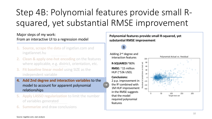
plt.show()10. Adding complexity to the model
Challenge, and try POLYNOMIAL features combined with LASSO, given the following observations: - the model is (slightly) overpredicting for prices ~60-75M HUF and underpredicting above (need for 2 ensemled models - not in scope) - the model might be missing polynomial and interdependency features (need for more features?)
Adding second degree polynomials to the model
# To avoid overfitting, creating polynomial terms for selected columns only
# A: function to add second degree term
def add_square_terms(df, selected_columns):

    df_poly = df.copy()

    for c in df.loc[:,selected_columns].columns:
        df_poly[c + '**2'] = df[c]**2

    return df_poly
Fitting polynomial model
# B: fitting polynomial model for selected columns
selected_columns = ['SIZE', 'FLOOR','FLOORS_IN_BUILDING','RELATIVE_FLOOR', 'DISTANCE_FROM_CENTRE','HALF_ROOMS','STANDARD_ROOMS','YOY_PERCENTAGE','AVG_PRICE']

X_train_poly = add_square_terms(X_train,selected_columns)
X_val_poly = add_square_terms(X_val,selected_columns)
X_test_poly = add_square_terms(X_test,selected_columns)

lm_poly = LinearRegression()
lm_poly.fit(X_train_poly, y_train)

test_set_pred_second = lm_poly.predict(X_test_poly)

print('Degree 2 polynomial regression validation R^2: %.3f', lm_poly.score(X_val_poly, y_val))
print('LINEAR regression validation R^2:', lr_model_linear.score(X_val, y_val))

print('Degree 2 polynomial regression test R^2: %.3f', lm_poly.score(X_test_poly, y_test))
print('LINEAR regression test R^2:', lr_model_linear.score(X_test, y_test))

print('2nd degree RMSE:',np.sqrt(mean_squared_error(y_test, test_set_pred_second)), 'MAE',mean_absolute_error(y_test,test_set_pred_second))
Applying LASSO regularization on polynomial model
# Pulling "back" polynomial model
# 1. Applying scaler
scaler = StandardScaler()
X_train_scaled = scaler.fit_transform(X_train_poly)
X_test_scaled = scaler.transform(X_test_poly)

## 2. Finding the "best" value of lambda (alpha) with a single train/valid split
alphalist = 10**(np.linspace(-3,4,200))
err_vec_val = np.zeros(len(alphalist))
err_vec_train = np.zeros(len(alphalist))

for i,curr_alpha in enumerate(alphalist):

    steps = [('standardize', StandardScaler()), ('lasso', Lasso(alpha = curr_alpha))]
#   steps = [('standardize', StandardScaler()), ('ridge', Ridge(alpha = curr_alpha))]

    pipe = Pipeline(steps)
    pipe.fit(X_train_poly, y_train)
    val_set_pred_lasso = pipe.predict(X_val_poly)
    err_vec_val[i] = np.sqrt(np.mean((val_set_pred_lasso - y_val)**2))

    train_set_pred_lasso = pipe.predict(X_train_poly)
    err_vec_train[i] = np.sqrt(np.mean((train_set_pred_lasso - y_train)**2))

# 3. This is the value of alpha that gave us the lowest error
ideal_alpha = alphalist[np.argmin(err_vec_val)]
print('Ideal alpha for LASSO', ideal_alpha)
Refitting regularized polynomial model
# 4. Fit the lasso model with above alpha
lr_model_lasso = Lasso(alpha = ideal_alpha)
lr_model_lasso.fit(X_train_scaled,y_train)

# 5. Predict on test data with LASSO model
test_set_pred_lasso = lr_model_lasso.predict(X_test_scaled)

# 6. Error testing
print(np.sqrt(mean_squared_error(y_test, test_set_pred_lasso)), mean_absolute_error(y_test,test_set_pred_lasso))

# 7. Final R**2 result and listing listing variables with statistical significance
print('LASSO regression test R^2:', lr_model_lasso.score(X_test_scaled, y_test))
print('Intercept:',lr_model_lasso.intercept_)

list(zip(X_train_poly.columns,lr_model_lasso.coef_))

#list(zip(poly.get_feature_names(),lr_model_lasso.coef_)) #to be used with polynomialfeatures()
Adding interaction features and polynomial features
# To avoid overfitting, creating polynomial terms for selected columns only
# A: function to add interaction terms of selected columns
def add_interaction_terms(df, selected_columns):

    df_poly = df.copy()

    interactions = PolynomialFeatures(degree=2, interaction_only=True)

    X_inter = interactions.fit_transform(df_poly.loc[:,selected_columns])
    target_feature_names = ['x'.join(['{}^{}'.format(pair[0],pair[1]) for pair in tuple if pair[1]!=0]) for tuple in [zip(df_poly.columns,p) for p in interactions.powers_]]

    X_inter = pd.DataFrame(X_inter,columns=target_feature_names)
    df_poly = X_inter.join(df_poly.reset_index())

    df_poly.drop(df_poly.columns[range(0, len(selected_columns)+1)], axis=1, inplace=True)
    del df_poly['index']

    return df_poly
interactions = PolynomialFeatures(degree=2, interaction_only=True)
lm_interaction = LinearRegression()
selected_columns_second_degree = ['SIZE', 'FLOOR','FLOORS_IN_BUILDING','RELATIVE_FLOOR', 'DISTANCE_FROM_CENTRE','HALF_ROOMS','STANDARD_ROOMS','YOY_PERCENTAGE','AVG_PRICE']
X_train_poly = add_interaction_terms(add_square_terms(X_train,selected_columns_second_degree),list(X_train.columns))
X_val_poly = add_interaction_terms(add_square_terms(X_val,selected_columns_second_degree),list(X_train.columns))
X_test_poly = add_interaction_terms(add_square_terms(X_test,selected_columns_second_degree),list(X_train.columns))
lm_interaction.fit(X_train_poly, y_train)
# 5. Predict on test data
test_set_pred_polynom = lm_interaction.predict(X_test_poly)
# 6. Error testing
print(np.sqrt(mean_squared_error(y_test, test_set_pred_polynom)), mean_absolute_error(y_test,test_set_pred_polynom))
print('Polynomial and interaction model R^2: %.3f' % lm_interaction.score(X_val_poly, y_val))
#list(zip(X_train_poly.columns,lm_interaction.coef_))## Residual Plot
## Plot predicted vs actual
plt.scatter(y_test,y_test-test_set_pred_polynom,alpha=.1)
plt.plot(np.linspace(0,150,1000),np.linspace(0,0,1000))
plt.title('Polynomial Actual vs. Residual')
plt.xlabel('Target test set')
plt.ylabel('Residual of predictions on test set')Applying regularization on interaction+polynomial model
In this regularization step I am using less verbose, yet more effective way to find the optimal alpha and fit regularized model in 1 step
# 1. Simpler LASSO methodology

scaler = StandardScaler()
X_train_scaled = scaler.fit_transform(X_train_poly)
X_test_scaled = scaler.transform(X_test_poly)

#alphavec = 10**np.linspace(-2,9,100)
lr_model_lasso = LassoCV(n_alphas=100, cv=5) #alphas = alphavec

lr_model_lasso.fit(X_train_scaled,y_train)

test_set_pred_lasso = lr_model_lasso.predict(X_test_scaled)
# 2. Error testing
print('RMSE:',np.sqrt(mean_squared_error(y_test, test_set_pred_lasso)), 'MAE:',mean_absolute_error(y_test,test_set_pred_lasso))
# 3. Final R**2 result and listing listing variables with statistical significance
print('LASSO regression train R^2:', lr_model_lasso.score(X_train_scaled, y_train))
print('LASSO regression test R^2:', lr_model_lasso.score(X_test_scaled, y_test))
print('Intercept:',lr_model_lasso.intercept_)
list(zip(X_train_poly.columns,lr_model_lasso.coef_))df_predictors = pd.DataFrame(list(zip(X_train_poly.columns,lr_model_lasso.coef_)),columns=['Predictor','Value'])
df_predictors['absolute_value'] = np.absolute(df_predictors['Value'])
print('Total features',df_predictors.Predictor.nunique())
df_predictors = df_predictors[df_predictors['Value'] != 0]
print('Relevant features',df_predictors.Predictor.nunique())
df_predictors.sort_values('absolute_value',ascending=False).head(10)Evaluate model performance
# Plot predicted vs actual
plt.scatter(test_set_pred_lasso,y_test,alpha=.1)
plt.plot(np.linspace(0,120,1000),np.linspace(5,100,1000))
## Residual Plot
## Plot predicted vs actual
plt.scatter(y_test,y_test-test_set_pred_lasso,alpha=.1)
plt.plot(np.linspace(0,150,1000),np.linspace(0,0,1000))
plt.title('LASSO Actual vs. Residual')
plt.xlabel('Target test set')
plt.ylabel('Residual of predictions on test set')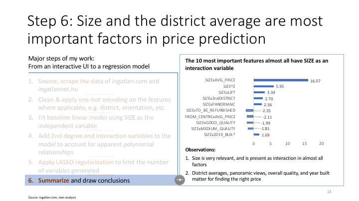

Additional options
In the below code you can see an example how the webscraping could have been conducted using selenium browser automation, instead of using beautifulsoup. Selenium comes handy when the website’s html does not have all the required information statically (e.g. login required, lazy loading of pictures, etc.)
Below the code is scrolling down the opened url to load lazy loading pics.
# Uses selenium to open the url, scroll to the bottom and return soup object
# not in use, given the slow speed of selenium
def site_to_soup(url):
    browser = webdriver.Chrome()
    browser.get(url)
    lenOfPage = browser.execute_script("window.scrollTo(0, document.body.scrollHeight);var lenOfPage=document.body.scrollHeight;return lenOfPage;")
    match=False
    while(match==False):
            lastCount = lenOfPage
            time.sleep(3)
            lenOfPage = browser.execute_script("window.scrollTo(0, document.body.scrollHeight);var lenOfPage=document.body.scrollHeight;return lenOfPage;")
            if lastCount==lenOfPage:
                match=True
    soup = BeautifulSoup(browser.page_source,"lxml")
    browser.quit()
    return soup