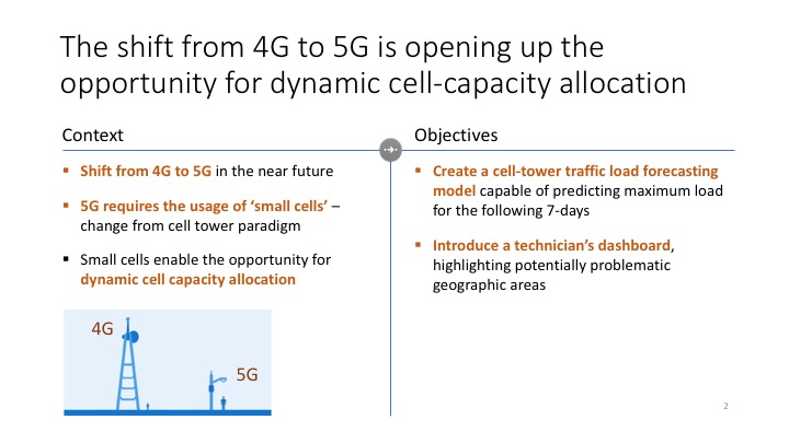
Dynamic cell-capacity allocation for telecoms
This project has served as my ‘passion-project’ in Metis Data Science Bootcamp in December, 2018 in New York.
# Plotting libraries
import geojson
import matplotlib.colors as colors
import matplotlib.cm as cmx
import seaborn as sns
%matplotlib inline
import matplotlib.pyplot as plt
from descartes import PolygonPatch
import matplotlib.animation as animation

# Standard libraries
import pandas as pd
import numpy as np

# Misc libraries
import json
import io
import requests

%matplotlib inline
1. Loading and Previewing the Data
Importing daily data from the Milando grid traffic, and aggregating into a single dataframe
import glob
import datetime
convert = lambda x: datetime.datetime.fromtimestamp(float(x) / 1e3)

df_cdrs = pd.DataFrame({})
colnames = ['CellID', 'datetime', 'countrycode','smsin','smsout', 'callin','callout', 'internet']
for filepath in glob.iglob('../01_Data/*.txt'):
    df = pd.read_csv(filepath, sep='\t', names=colnames,parse_dates=['datetime'], date_parser=convert)
    df_cdrs = df_cdrs.append(df)
    print(f'Finished {filepath}')
#df_cdrs.to_pickle('raw_merged.pkl')
Finished ../01_Data/01_November_Data/sms-call-internet-mi-2013-11-25.txt
Finished ../01_Data/01_November_Data/sms-call-internet-mi-2013-11-19.txt
Finished ../01_Data/01_November_Data/sms-call-internet-mi-2013-11-18.txt
Finished ../01_Data/01_November_Data/sms-call-internet-mi-2013-11-30.txt
Finished ../01_Data/01_November_Data/sms-call-internet-mi-2013-11-24.txt
Finished ../01_Data/01_November_Data/sms-call-internet-mi-2013-11-26.txt
Finished ../01_Data/01_November_Data/sms-call-internet-mi-2013-11-27.txt
Aggregating milano grid traffic to a max of (sum of hourly) traffic for each day. Assuming that a single call/internet connection can last on avarage for a max of hour - and the cell tower has to be able to serve the highest traffic of the highest hour
df_cdrs=df_cdrs.fillna(0)
df_cdrs['sms'] = df_cdrs['smsin'] + df_cdrs['smsout']
df_cdrs['calls'] = df_cdrs['callin'] + df_cdrs['callout']
df_cdrs = (df_cdrs[['datetime', 'CellID', 'internet', 'calls', 'sms']].set_index('datetime')
             .groupby([pd.Grouper(freq='H'),'CellID']).sum().reset_index().set_index('datetime')
             .groupby([pd.Grouper(freq='D'),'CellID']).max()
            )
df_cdrs.index.names = ['day', 'CellID']
df_cdrs.reset_index(inplace=True)
#df_cdrs.to_pickle('group_merged.pkl')
#for day_df in df_cdrs.groupby(['day']):
    #break
Running the above on AWS, importing locally and cleaning
def import_source_data(filepath):
    df_cdrs = pd.read_csv(filepath)
    del df_cdrs['Unnamed: 0']

    return df_cdrs
For a detailed visual representation of the data, visit: https://public.tableau.com/profile/krisztian.sandor#!/vizhome/Kojak_v1_1/Dashboard1
2. Train and Validation Series Partioning
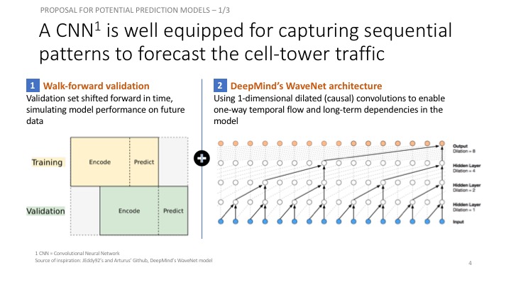
We’ll use a style of walk-forward validation, where our validation set spans the same time-range as our training set, but shifted forward in time (in this case by 14 days). This way, we simulate how our model will perform on unseen data that comes in the future.
df_cdrs = import_source_data('../01_Data/03_AWS outputs/group_merged.csv')

from datetime import timedelta

pred_steps = 7 # Predicting the max of next 7 days
pred_length=timedelta(pred_steps)

data_start_date = df_cdrs.day.min()
data_end_date = df_cdrs.day.max()
print('Data ranges from %s to %s' % (data_start_date, data_end_date))

first_day = pd.to_datetime(data_start_date)
last_day = pd.to_datetime(data_end_date)

val_pred_start = last_day - pred_length + timedelta(1)
val_pred_end = last_day

train_pred_start = val_pred_start - pred_length
train_pred_end = val_pred_start - timedelta(days=1)

enc_length = train_pred_start - first_day

train_enc_start = first_day
train_enc_end = train_enc_start + enc_length - timedelta(1)

val_enc_start = train_enc_start + pred_length
val_enc_end = val_enc_start + enc_length - timedelta(1)

print('Train encoding:', train_enc_start, '-', train_enc_end)
print('Train prediction:', train_pred_start, '-', train_pred_end, '\n')
print('Val encoding:', val_enc_start, '-', val_enc_end)
print('Val prediction:', val_pred_start, '-', val_pred_end)

print('\nEncoding interval:', enc_length.days)
print('Prediction interval:', pred_length.days)
Data ranges from 2013-10-31 to 2014-01-01
Train encoding: 2013-10-31 00:00:00 - 2013-12-18 00:00:00
Train prediction: 2013-12-19 00:00:00 - 2013-12-25 00:00:00
Val encoding: 2013-11-07 00:00:00 - 2013-12-25 00:00:00
Val prediction: 2013-12-26 00:00:00 - 2014-01-01 00:00:00
Encoding interval: 49
Prediction interval: 7
3. Keras Data Formatting
Now that we have the time segment dates, we’ll define the functions we need to extract the data in keras friendly format. Here are the steps: - Pull the time series into an array, save a date_to_index mapping as a utility for referencing into the array - Create function to extract specified time interval from all the series - Create functions to transform all the series. - Here we smooth out the scale by taking log1p and de-meaning each series using the encoder series mean, then reshape to the (n_series, n_timesteps, n_features) tensor format that keras will expect. - Note that if we want to generate true predictions instead of log scale ones, we can easily apply a reverse transformation at prediction time.
df_pivoted = pd.pivot_table(df_cdrs, values='internet', index='CellID', columns='day', aggfunc=np.sum)
date_to_index = pd.Series(index=pd.Index([pd.to_datetime(c) for c in df_pivoted.columns]),
                          data=[i for i in range(len(df_pivoted.columns))])

series_array = df_pivoted.values
def get_time_block_series(series_array, date_to_index, start_date, end_date):
inds = date_to_index[start_date:end_date]
return series_array[:,inds]
def transform_series_encode(series_array):
series_array = np.log1p(np.nan_to_num(series_array)) # filling NaN with 0
series_mean = series_array.mean(axis=1).reshape(-1,1)
series_array = series_array - series_mean
series_array = series_array.reshape((series_array.shape[0],series_array.shape[1], 1))
return series_array, series_mean
def transform_series_decode(series_array, encode_series_mean):
series_array = np.log1p(np.nan_to_num(series_array)) # filling NaN with 0
series_array = series_array - encode_series_mean
series_array = series_array.reshape((series_array.shape[0],series_array.shape[1], 1))
return series_array4. CNN Architecture
- 8 dilated causal convolutional layers
- 32 filters of width 2 per layer
- Exponentially increasing dilation rate (1, 2, 4, 8, …, 128)
- 2 (time distributed) fully connected layers to map to final output
We’ll extract the last 7 steps from the output sequence as our predicted output for training. We’ll use teacher forcing again during training. We’ll have a separate function that runs an inference loop to generate predictions on unseen data, iteratively filling previous predictions into the history sequence.
This convolutional architecture is a simplified version of the WaveNet model, designed as a generative model for audio (in particular, for text-to-speech applications). The wavenet model can be abstracted beyond audio to apply to any time series forecasting problem, providing a nice structure for capturing long-term dependencies without an excessive number of learned weights. The core building block of the wavenet model is the dilated causal convolution layer. It utilizes some other key techniques like gated activations and skip connections, but for now we’ll focus on the central idea of the architecture to keep things simple (check out the next notebook in the series for these). I’ll explain this style of convolution (causal and dilated), then show how to implement our simplified WaveNet architecture in keras.
Causal Convolutions
In a traditional 1-dimensional convolution layer, as in the image below taken from Chris Olah’s excellent blog, we slide a filter of weights across an input series, sequentially applying it to (usually overlapping) regions of the series. The output shape will depend on the sequence padding used, and is closely related to the connection structure between inputs and outputs. In this example, a filter of width 2, stride of 1, and no padding means that the output sequence will have one fewer entry than the input.
1dconv
In the image, imagine that $y_0,…, y_7$ are each prediction outputs for the time steps that follow the series values $x_0,…,x_7$. There is a clear problem - since $x_1$ influences the output $y_0$, we would be using the future to predict the past, which is cheating! Letting the future of a sequence influence our interpretation of its past makes sense in a context like text classification where we use a known sequence to predict an outcome, but not in our time series context where we must generate future values in a sequence.
To solve this problem, we adjust our convolution design to explicitly prohibit the future from influencing the past. In other words, we only allow inputs to connect to future time step outputs in a causal structure, as pictured below in a visualization from the WaveNet paper. In practice, this causal 1D structure is easy to implement by shifting traditional convolutional outputs by a number of timesteps. Keras handles it via setting padding = ‘causal’.
causalconv
Dilated (Causal) Convolutions
With causal convolutions we have the proper tool for handling temporal flow, but we need an additional modification to properly handle long-term dependencies. In the simple causal convolution figure above, you can see that only the 5 most recent timesteps can influence the highlighted output. In fact, we would require one additional layer per timestep to reach farther back in the series (to use proper terminology, to increase the output’s receptive field). With a time series that extends for over a year, using simple causal convolutions to learn from the entire history would quickly make our model way too computationally and statistically complex.
Instead of making that mistake, WaveNet uses dilated convolutions, which allow the receptive field to increase exponentially as a function of the number of convolutional layers. In a dilated convolution layer, filters are not applied to inputs in a simple sequential manner, but instead skip a constant dilation rate inputs in between each of the inputs they process, as in the WaveNet diagram below. By increasing the dilation rate multiplicatively at each layer (e.g. 1, 2, 4, 8, …), we can achieve the exponential relationship between layer count and receptive field size that we desire. In the diagram, you can see how we now only need 4 layers to connect all of the 16 input series values to the highlighted output (say the 17th time step value).
from keras.models import Model
from keras.layers import Input, Conv1D, Dense, Dropout, Lambda, concatenate
from keras.optimizers import Adam
from keras.callbacks import EarlyStopping

# convolutional layer parameters
n_filters = 32
filter_width = 2
dilation_rates = [2**i for i in range(8)]

# define an input history series and pass it through a stack of dilated causal convolutions.
history_seq = Input(shape=(None, 1))
x = history_seq

for dilation_rate in dilation_rates:
    x = Conv1D(filters=n_filters,
               kernel_size=filter_width,
               padding='causal',
               dilation_rate=dilation_rate)(x)

x = Dense(128, activation='relu')(x)
x = Dropout(.2)(x)
x = Dense(1)(x)

# extract the last 7 time steps as the training target
def slice(x, seq_length):
    return x[:,-seq_length:,:]

pred_seq_train = Lambda(slice, arguments={'seq_length':pred_steps})(x)

model = Model(history_seq, pred_seq_train)
Using TensorFlow backend.
model.summary()_________________________________________________________________
Layer (type) Output Shape Param #
=================================================================
input_1 (InputLayer) (None, None, 1) 0
_________________________________________________________________
conv1d_1 (Conv1D) (None, None, 32) 96
_________________________________________________________________
conv1d_2 (Conv1D) (None, None, 32) 2080
_________________________________________________________________
conv1d_3 (Conv1D) (None, None, 32) 2080
_________________________________________________________________
conv1d_4 (Conv1D) (None, None, 32) 2080
_________________________________________________________________
conv1d_5 (Conv1D) (None, None, 32) 2080
_________________________________________________________________
conv1d_6 (Conv1D) (None, None, 32) 2080
_________________________________________________________________
conv1d_7 (Conv1D) (None, None, 32) 2080
_________________________________________________________________
conv1d_8 (Conv1D) (None, None, 32) 2080
_________________________________________________________________
dense_1 (Dense) (None, None, 128) 4224
_________________________________________________________________
dropout_1 (Dropout) (None, None, 128) 0
_________________________________________________________________
dense_2 (Dense) (None, None, 1) 129
_________________________________________________________________
lambda_1 (Lambda) (None, None, 1) 0
=================================================================
Total params: 19,009
Trainable params: 19,009
Non-trainable params: 0
_________________________________________________________________
first_n_samples = 40000 # no effect
batch_size = 2**11
epochs = 1000

# sample of series from train_enc_start to train_enc_end
encoder_input_data = get_time_block_series(series_array, date_to_index,
                                           train_enc_start, train_enc_end)[:first_n_samples]
encoder_input_data, encode_series_mean = transform_series_encode(encoder_input_data)

# sample of series from train_pred_start to train_pred_end
decoder_target_data = get_time_block_series(series_array, date_to_index,
                                            train_pred_start, train_pred_end)[:first_n_samples]
decoder_target_data = transform_series_decode(decoder_target_data, encode_series_mean)

# we append a lagged history of the target series to the input data,
# so that we can train with teacher forcing
lagged_target_history = decoder_target_data[:,:-1,:1]
encoder_input_data = np.concatenate([encoder_input_data, lagged_target_history], axis=1)model.compile(Adam(), loss='mean_absolute_error')
monitor = EarlyStopping(monitor='val_loss', min_delta=1e-3, patience=5, verbose=1, mode='auto')
history = model.fit(encoder_input_data, decoder_target_data,
batch_size=batch_size,
callbacks=[monitor],
epochs=epochs,
validation_split=0.2)Train on 8000 samples, validate on 2000 samples
Epoch 1/1000
8000/8000 [==============================] - 7s 892us/step - loss: 0.2658 - val_loss: 0.1406
Epoch 2/1000
8000/8000 [==============================] - 6s 750us/step - loss: 0.2148 - val_loss: 0.1575
Epoch 3/1000
8000/8000 [==============================] - 6s 747us/step - loss: 0.1953 - val_loss: 0.1216
Epoch 4/1000
8000/8000 [==============================] - 6s 755us/step - loss: 0.1824 - val_loss: 0.1180
Epoch 5/1000
8000/8000 [==============================] - 6s 752us/step - loss: 0.1693 - val_loss: 0.1225
Epoch 6/1000
8000/8000 [==============================] - 6s 756us/step - loss: 0.1584 - val_loss: 0.1071
Epoch 7/1000
8000/8000 [==============================] - 6s 754us/step - loss: 0.1493 - val_loss: 0.1136
Epoch 8/1000
8000/8000 [==============================] - 6s 752us/step - loss: 0.1446 - val_loss: 0.1077
Epoch 9/1000
8000/8000 [==============================] - 6s 748us/step - loss: 0.1411 - val_loss: 0.1071
Epoch 10/1000
8000/8000 [==============================] - 6s 754us/step - loss: 0.1383 - val_loss: 0.1056
Epoch 11/1000
8000/8000 [==============================] - 6s 753us/step - loss: 0.1360 - val_loss: 0.1047
Epoch 12/1000
8000/8000 [==============================] - 6s 754us/step - loss: 0.1346 - val_loss: 0.1037
Epoch 13/1000
8000/8000 [==============================] - 6s 752us/step - loss: 0.1329 - val_loss: 0.1045
Epoch 14/1000
8000/8000 [==============================] - 6s 752us/step - loss: 0.1319 - val_loss: 0.1022
Epoch 15/1000
8000/8000 [==============================] - 6s 750us/step - loss: 0.1307 - val_loss: 0.1039
Epoch 16/1000
8000/8000 [==============================] - 6s 749us/step - loss: 0.1302 - val_loss: 0.1018
Epoch 17/1000
8000/8000 [==============================] - 6s 753us/step - loss: 0.1294 - val_loss: 0.1017
Epoch 18/1000
8000/8000 [==============================] - 6s 751us/step - loss: 0.1288 - val_loss: 0.1026
Epoch 19/1000
8000/8000 [==============================] - 6s 750us/step - loss: 0.1284 - val_loss: 0.1010
Epoch 20/1000
8000/8000 [==============================] - 6s 754us/step - loss: 0.1275 - val_loss: 0.1017
Epoch 21/1000
8000/8000 [==============================] - 6s 752us/step - loss: 0.1269 - val_loss: 0.1015
Epoch 22/1000
8000/8000 [==============================] - 6s 755us/step - loss: 0.1269 - val_loss: 0.1008
Epoch 23/1000
8000/8000 [==============================] - 6s 749us/step - loss: 0.1263 - val_loss: 0.1007
Epoch 24/1000
8000/8000 [==============================] - 6s 751us/step - loss: 0.1259 - val_loss: 0.1002
Epoch 00024: early stopping
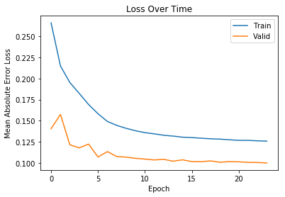
plt.plot(history.history['loss'])
plt.plot(history.history['val_loss'])
plt.xlabel('Epoch')
plt.ylabel('Mean Absolute Error Loss')
plt.title('Loss Over Time')
plt.legend(['Train','Valid'])<matplotlib.legend.Legend at 0x7f8dc9d3b320>
# Save model to disk
model_name='model_1f'
# serialize model to JSON
model_json = model.to_json()
with open(model_name+".json", "w") as json_file:
json_file.write(model_json)
# serialize weights to HDF5
model.save_weights(model_name+".h5")
print(f"Saved {model_name} to disk")Saved model_1f to disk
# Load model from disk if already saved
def import_model(model_name):
from keras.models import model_from_json
# load json and create model
json_file = open(model_name+'.json', 'r')
loaded_model_json = json_file.read()
json_file.close()
loaded_model = model_from_json(loaded_model_json)
# load weights into new model
loaded_model.load_weights(model_name+".h5")
print(f"Loaded {model_name} from disk")
return loaded_model5. Building the Model - Inference Loop
The model outputs the next 7 time predictions. We are only using the first prediction each time, the rest is used for teacher forcing. Teacher forcing is a methodology to use most recent predictions of the model for predicting the next period, i.e. learn from its mistakes.
def predict_sequence_1f(input_sequence, model):
history_sequence = input_sequence.copy()
pred_sequence = np.zeros((1,pred_steps,1)) # initialize output (pred_steps time steps)
for i in range(pred_steps):
# record next time step prediction (last time step of model output)
last_step_pred = model.predict(history_sequence)[0,-1,0]
pred_sequence[0,i,0] = last_step_pred
# add the next time step prediction to the history sequence
history_sequence = np.concatenate([history_sequence,
last_step_pred.reshape(-1,1,1)], axis=1)
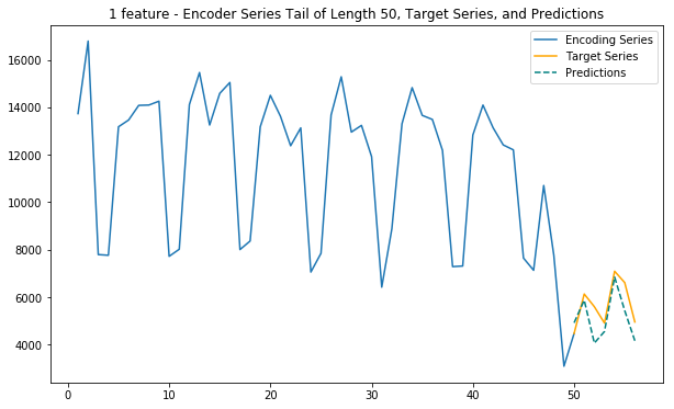
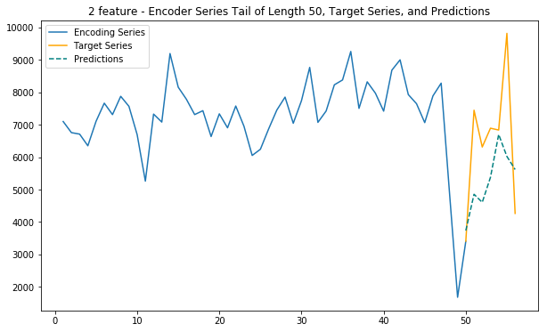
return pred_sequence6. Generating and Plotting Predictions
encoder_input_data = get_time_block_series(series_array, date_to_index, val_enc_start, val_enc_end)
encoder_input_data, encode_series_mean = transform_series_encode(encoder_input_data)
decoder_target_data = get_time_block_series(series_array, date_to_index, val_pred_start, val_pred_end)
decoder_target_data = transform_series_decode(decoder_target_data, encode_series_mean)def predict_and_plot(encoder_input_data, decoder_target_data, sample_ind, encode_series_mean, model, enc_tail_len=50):
sample_ind -= 1
encode_series = encoder_input_data[sample_ind:sample_ind+1,:,:]
pred_series = predict_sequence_1f(encode_series,model)
encode_series = np.expm1(encode_series.reshape(-1,1) + encode_series_mean[sample_ind])
pred_series = np.expm1(pred_series.reshape(-1,1) + encode_series_mean[sample_ind])
target_series = np.expm1(decoder_target_data[sample_ind,:,:1].reshape(-1,1) + encode_series_mean[sample_ind])
encode_series_tail = np.concatenate([encode_series[-enc_tail_len:],target_series[:1]])
x_encode = encode_series_tail.shape[0]
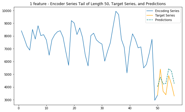
plt.figure(figsize=(10,6))
plt.plot(range(1,x_encode+1),encode_series_tail)
plt.plot(range(x_encode,x_encode+pred_steps),target_series,color='orange')
plt.plot(range(x_encode,x_encode+pred_steps),pred_series,color='teal',linestyle='--')
plt.title('1 feature - Encoder Series Tail of Length %d, Target Series, and Predictions' % enc_tail_len)
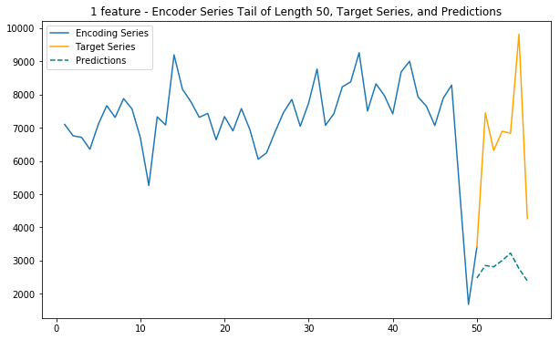
plt.legend(['Encoding Series','Target Series','Predictions'])6. Main function (1 feature)
This function uses only internet traffic as input variable to predict future internet traffic
def main_1(cell_id):
# Main 1 feature model
model_to_use = '../01_Data/03_AWS outputs/model_1f'
# Import model
df_cdrs = import_source_data('../01_Data/03_AWS outputs/group_merged.csv')
model = import_model(model_to_use)
# Format data
df_pivoted = pd.pivot_table(df_cdrs, values='internet', index='CellID', columns='day', aggfunc=np.sum)
date_to_index = pd.Series(index=pd.Index([pd.to_datetime(c) for c in df_pivoted.columns]),
data=[i for i in range(len(df_pivoted.columns))])
series_array = df_pivoted.values
# Generate encoder and decoder dataset
encoder_input_data = get_time_block_series(series_array, date_to_index, val_enc_start, val_enc_end)
encoder_input_data, encode_series_mean = transform_series_encode(encoder_input_data)
decoder_target_data = get_time_block_series(series_array, date_to_index, val_pred_start, val_pred_end)
decoder_target_data = transform_series_decode(decoder_target_data, encode_series_mean)
# Predict and plot
predict_and_plot(encoder_input_data, decoder_target_data, cell_id, encode_series_mean, model=model)7. Integrating calls and sms features
The previous model only used the historical internet traffic to predict the future internet traffic. Here we are extending the model to take the historical calls and sms traffic besides the internet traffic to generate predictions
df_cdrs.head()| day | CellID | internet | calls | sms | |
|---|---|---|---|---|---|
| 0 | 2013-10-31 | 1 | 57.799009 | 1.021221 | 3.189034 |
| 1 | 2013-10-31 | 2 | 57.914858 | 1.040205 | 3.179480 |
| 2 | 2013-10-31 | 3 | 58.038173 | 1.060412 | 3.169311 |
| 3 | 2013-10-31 | 4 | 57.463453 | 0.966233 | 3.216705 |
| 4 | 2013-10-31 | 5 | 52.171423 | 0.884973 | 2.914617 |
df_cdrs = import_source_data('../01_Data/03_AWS outputs/group_merged.csv')8. Re-scale each feature separatly
Re-scaling each feature (internet, calls, sms) separately for each cell separately captures the various patterns in the series
def agg_func(col):
global mean_list
log_c=np.log1p(col)
mean_log_c=np.mean(np.log1p(col))
mean_list.append(np.array(mean_log_c))
return log_c-mean_log_c
def scaler(df_cdrs,dim):
global mean_list
for col_name in df_cdrs.columns[2:2+dim]:
#print(col_name)
df_cdrs[col_name+'_scaled'] = df_cdrs.groupby(['CellID'])[col_name].apply(agg_func)
cells = df_cdrs.CellID.nunique()
means=np.zeros((10000,dim))
for i in range(dim):
means[:,i] = np.array(mean_list[i*cells:(i+1)*cells])
mean_list = means
return df_cdrs, mean_listdf_cdrs.head()| day | CellID | internet | calls | sms | internet_scaled | calls_scaled | sms_scaled | |
|---|---|---|---|---|---|---|---|---|
| 0 | 2013-10-31 | 1 | 57.799009 | 1.021221 | 3.189034 | -0.477102 | -1.855503 | -1.144778 |
| 1 | 2013-10-31 | 2 | 57.914858 | 1.040205 | 3.179480 | -0.479278 | -1.860002 | -1.160078 |
| 2 | 2013-10-31 | 3 | 58.038173 | 1.060412 | 3.169311 | -0.481585 | -1.864703 | -1.176392 |
| 3 | 2013-10-31 | 4 | 57.463453 | 0.966233 | 3.216705 | -0.470914 | -1.841838 | -1.099484 |
| 4 | 2013-10-31 | 5 | 52.171423 | 0.884973 | 2.914617 | -0.468362 | -1.819482 | -1.106134 |
9. Reformat data for KERAS
Keras Conv1D requires 3 dimensional input data (samples=cell-towers, dates, features)
# VERY INEFFICIENT way to create keras friendly data format
from IPython.display import clear_output
# Building KERAS friendly data in the dimensions (n_celltowers, dates, features):(10000,63,3)
x = df_cdrs.CellID.nunique()
y, y_list = df_cdrs.day.nunique(), df_cdrs.day.unique()
d_dates_index = dict(zip(y_list,range(y)))
z = dim
keras_matrix = np.zeros((x,y,z))
for name,group in df_cdrs.groupby(['CellID'])['internet_scaled','calls_scaled','sms_scaled']:
status = round(name/x*100)
clear_output()
print(f'Progress: {status}%')
group[name] = group[group.columns[2:2+dim]].values.tolist()
group = group[['day',name]]
group.set_index(['day'],inplace=True)
for date in y_list:
if date in group.index:
for f in range(z):
keras_matrix[name-1][d_dates_index[date]][f]=group.loc[date].values[0][f]
keras_matrix.dump("keras_matrix_newscaling.dat")Progress: 100%
# This is a MUCH faster reformatting algorithm for KERAS inputs
def create_keras_matrix(df_cdrs,dim):
l=[]
for n,v in df_cdrs.groupby(['CellID']):
#print(n)
cell_data = v[v.columns[2+dim:]].values
if cell_data.shape[0] != 63:
# for missing dates use mean of rest
sub = np.array([cell_data[:,i].mean() for i in range(dim)]).reshape(1,dim)
for i in range(0,63-cell_data.shape[0]):
cell_data = np.append(cell_data,sub)
cell_data = cell_data.reshape(63,dim)
l.append(cell_data)
keras_matrix = np.array(l)
keras_matrix.dump("keras_matrix_internet+zones_featurenr_"+str(dim)+".dat")
return keras_matrixcreate_keras_matrix(df_cdrs,dim)keras_matrix = np.load("../01_Data/03_AWS outputs/keras_matrix_newscaling.dat")
y, y_list = df_cdrs.day.nunique(), df_cdrs.day.unique()
d_dates_index = dict(zip(y_list,range(y)))# data from train_enc_start to train_enc_end
encoder_input_data = (keras_matrix
[:, # all cell-towers
d_dates_index[train_enc_start.strftime('%Y-%m-%d')]: # start of training period
d_dates_index[train_enc_end.strftime('%Y-%m-%d')]+1, # end of training period
:] # all features
)
# data from train_pred_start to train_pred_end
decoder_target_data = (keras_matrix
[:, # all cell-towers
d_dates_index[train_pred_start.strftime('%Y-%m-%d')]: # start of pred period
d_dates_index[train_pred_end.strftime('%Y-%m-%d')]+1, # end of pred period
:] # all features to be used as target
)
# we append a lagged history of the target series to the input data,
# so that we can train with teacher forcing
lagged_target_history = decoder_target_data[:,:-1,:]
encoder_input_data = np.concatenate([encoder_input_data, lagged_target_history], axis=1)from keras.models import Model
from keras.layers import Input, Conv1D, Dense, Dropout, Lambda, concatenate
from keras.optimizers import Adam
from keras.callbacks import EarlyStopping
# convolutional layer parameters
n_filters = 32
filter_width = 2
dilation_rates = [2**i for i in range(8)]
# define an input history series and pass it through a stack of dilated causal convolutions.
history_seq = Input(shape=(None, 3))
x = history_seq
for dilation_rate in dilation_rates:
x = Conv1D(filters=n_filters,
kernel_size=filter_width,
padding='causal',
dilation_rate=dilation_rate)(x)
x = Dense(128, activation='relu')(x)
x = Dropout(.2)(x)
x = Dense(3)(x)
# extract the last 7 time steps as the training target
def slice(x, seq_length):
return x[:,-seq_length:,:]
pred_seq_train = Lambda(slice, arguments={'seq_length':pred_steps})(x)
model = Model(history_seq, pred_seq_train)
model.summary()_________________________________________________________________
Layer (type) Output Shape Param #
=================================================================
input_2 (InputLayer) (None, None, 3) 0
_________________________________________________________________
conv1d_9 (Conv1D) (None, None, 32) 224
_________________________________________________________________
conv1d_10 (Conv1D) (None, None, 32) 2080
_________________________________________________________________
conv1d_11 (Conv1D) (None, None, 32) 2080
_________________________________________________________________
conv1d_12 (Conv1D) (None, None, 32) 2080
_________________________________________________________________
conv1d_13 (Conv1D) (None, None, 32) 2080
_________________________________________________________________
conv1d_14 (Conv1D) (None, None, 32) 2080
_________________________________________________________________
conv1d_15 (Conv1D) (None, None, 32) 2080
_________________________________________________________________
conv1d_16 (Conv1D) (None, None, 32) 2080
_________________________________________________________________
dense_3 (Dense) (None, None, 128) 4224
_________________________________________________________________
dropout_2 (Dropout) (None, None, 128) 0
_________________________________________________________________
dense_4 (Dense) (None, None, 3) 387
_________________________________________________________________
lambda_2 (Lambda) (None, None, 3) 0
=================================================================
Total params: 19,395
Trainable params: 19,395
Non-trainable params: 0
_________________________________________________________________
batch_size = 2**11
epochs = 100
model.compile(Adam(), loss='mean_absolute_error')
monitor = EarlyStopping(monitor='val_loss', min_delta=1e-3, patience=5, verbose=1, mode='auto')
history = model.fit(encoder_input_data, decoder_target_data,
                    batch_size=batch_size,
                    callbacks=[monitor],
                    epochs=epochs,
                    validation_split=0.2)
Train on 8000 samples, validate on 2000 samples
Epoch 1/100
8000/8000 [==============================] - 7s 892us/step - loss: 0.2787 - val_loss: 0.2107
Epoch 2/100
8000/8000 [==============================] - 6s 766us/step - loss: 0.2331 - val_loss: 0.1863
Epoch 3/100
8000/8000 [==============================] - 6s 768us/step - loss: 0.2049 - val_loss: 0.1714
Epoch 4/100
8000/8000 [==============================] - 6s 769us/step - loss: 0.1878 - val_loss: 0.1557
Epoch 5/100
8000/8000 [==============================] - 6s 766us/step - loss: 0.1779 - val_loss: 0.1418
Epoch 6/100
8000/8000 [==============================] - 6s 768us/step - loss: 0.1678 - val_loss: 0.1366
Epoch 7/100
8000/8000 [==============================] - 6s 782us/step - loss: 0.1615 - val_loss: 0.1307
Epoch 8/100
8000/8000 [==============================] - 6s 781us/step - loss: 0.1564 - val_loss: 0.1286
Epoch 9/100
8000/8000 [==============================] - 6s 775us/step - loss: 0.1526 - val_loss: 0.1242
Epoch 10/100
8000/8000 [==============================] - 6s 776us/step - loss: 0.1494 - val_loss: 0.1239
Epoch 11/100
8000/8000 [==============================] - 6s 773us/step - loss: 0.1466 - val_loss: 0.1220
Epoch 12/100
8000/8000 [==============================] - 6s 773us/step - loss: 0.1439 - val_loss: 0.1209
Epoch 13/100
8000/8000 [==============================] - 6s 770us/step - loss: 0.1418 - val_loss: 0.1201
Epoch 14/100
8000/8000 [==============================] - 6s 775us/step - loss: 0.1401 - val_loss: 0.1184
Epoch 15/100
8000/8000 [==============================] - 6s 780us/step - loss: 0.1382 - val_loss: 0.1171
Epoch 16/100
8000/8000 [==============================] - 6s 783us/step - loss: 0.1367 - val_loss: 0.1162
Epoch 17/100
8000/8000 [==============================] - 6s 789us/step - loss: 0.1353 - val_loss: 0.1164
Epoch 18/100
8000/8000 [==============================] - 6s 782us/step - loss: 0.1339 - val_loss: 0.1166
Epoch 19/100
8000/8000 [==============================] - 6s 777us/step - loss: 0.1328 - val_loss: 0.1151
Epoch 20/100
8000/8000 [==============================] - 6s 785us/step - loss: 0.1316 - val_loss: 0.1138
Epoch 21/100
8000/8000 [==============================] - 6s 780us/step - loss: 0.1306 - val_loss: 0.1136
Epoch 22/100
8000/8000 [==============================] - 6s 776us/step - loss: 0.1300 - val_loss: 0.1130
Epoch 23/100
8000/8000 [==============================] - 6s 772us/step - loss: 0.1290 - val_loss: 0.1129
Epoch 24/100
8000/8000 [==============================] - 6s 772us/step - loss: 0.1281 - val_loss: 0.1123
Epoch 25/100
8000/8000 [==============================] - 6s 771us/step - loss: 0.1272 - val_loss: 0.1121
Epoch 26/100
8000/8000 [==============================] - 6s 778us/step - loss: 0.1267 - val_loss: 0.1116
Epoch 27/100
8000/8000 [==============================] - 6s 791us/step - loss: 0.1261 - val_loss: 0.1104
Epoch 28/100
8000/8000 [==============================] - 6s 790us/step - loss: 0.1254 - val_loss: 0.1100
Epoch 29/100
8000/8000 [==============================] - 6s 786us/step - loss: 0.1251 - val_loss: 0.1094
Epoch 30/100
8000/8000 [==============================] - 6s 779us/step - loss: 0.1244 - val_loss: 0.1098
Epoch 31/100
8000/8000 [==============================] - 6s 780us/step - loss: 0.1237 - val_loss: 0.1090
Epoch 32/100
8000/8000 [==============================] - 6s 779us/step - loss: 0.1230 - val_loss: 0.1087
Epoch 33/100
8000/8000 [==============================] - 6s 779us/step - loss: 0.1226 - val_loss: 0.1085
Epoch 34/100
8000/8000 [==============================] - 6s 771us/step - loss: 0.1221 - val_loss: 0.1080
Epoch 35/100
8000/8000 [==============================] - 6s 774us/step - loss: 0.1217 - val_loss: 0.1082
Epoch 36/100
8000/8000 [==============================] - 6s 776us/step - loss: 0.1212 - val_loss: 0.1076
Epoch 37/100
8000/8000 [==============================] - 6s 779us/step - loss: 0.1209 - val_loss: 0.1076
Epoch 38/100
8000/8000 [==============================] - 6s 773us/step - loss: 0.1203 - val_loss: 0.1076
Epoch 39/100
8000/8000 [==============================] - 6s 784us/step - loss: 0.1198 - val_loss: 0.1078
Epoch 00039: early stopping
model_name='../01_Data/03_AWS outputs/model_3f_20181203_1651'
# serialize model to JSON
model_json = model.to_json()
with open(model_name+".json", "w") as json_file:
json_file.write(model_json)
# serialize weights to HDF5
model.save_weights(model_name+".h5")
print(f"Saved {model_name} to disk")Saved model_3f_20181203_1651 to disk
# Bulding predictions from n feature model
def predict_sequence_multi_f(input_sequence, model, dim):
history_sequence = input_sequence.copy()
pred_sequence = np.zeros((1,pred_steps,dim)) # initialize output (pred_steps time steps)
for i in range(pred_steps): #pred_steps=7 at beginning of code
# record next time step prediction (last time step of model output)
last_step_pred = model.predict(history_sequence)[0,-1,:]
pred_sequence[0,i,:] = last_step_pred
# add the next time step prediction to the history sequence
history_sequence = np.concatenate([history_sequence,
last_step_pred.reshape(-1,1,dim)], axis=1)
return pred_sequenceencoder_input_data = (keras_matrix
[:, # all cell-towers
d_dates_index[val_enc_start.strftime('%Y-%m-%d')]: # start of training period
d_dates_index[val_enc_end.strftime('%Y-%m-%d')]+1, # end of training period
:] # all features
)
# data from train_pred_start to train_pred_end
decoder_target_data = (keras_matrix
[:, # all cell-towers
d_dates_index[val_pred_start.strftime('%Y-%m-%d')]: # start of pred period
d_dates_index[val_pred_end.strftime('%Y-%m-%d')]+1, # end of pred period
:] # all features to be used as target
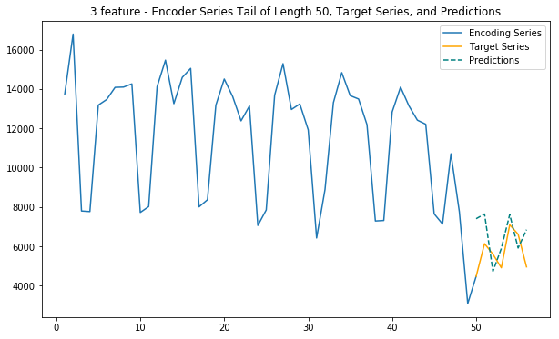
)def predict_and_plot_multi_f(encoder_input_data, decoder_target_data, sample_ind, mean_list, model, dim, enc_tail_len=50):
# e.g. Cell ID 1 is 0 in df
sample_ind -= 1
encode_series = encoder_input_data[sample_ind:sample_ind+1,:,:]
pred_series = predict_sequence_multi_f(encode_series, model, dim)
# Only use internet predictions for viz (col 0 --> :1)
encode_series = np.expm1(encode_series.reshape(-1,dim) + mean_list[sample_ind])[:,:1]
pred_series = np.expm1(pred_series.reshape(-1,dim) + mean_list[sample_ind])[:,:1]
target_series = np.expm1(decoder_target_data[sample_ind,:,:dim].reshape(-1,dim) + mean_list[sample_ind])[:,:1]
encode_series_tail = np.concatenate([encode_series[-enc_tail_len:],target_series[:1]])
x_encode = encode_series_tail.shape[0]
plt.figure(figsize=(10,6))
plt.plot(range(1,x_encode+1),encode_series_tail)
plt.plot(range(x_encode,x_encode+pred_steps),target_series,color='orange')
plt.plot(range(x_encode,x_encode+pred_steps),pred_series,color='teal',linestyle='--')
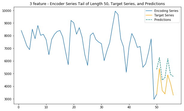
plt.title(f'{dim} feature - Encoder Series Tail of Length {enc_tail_len}, Target Series, and Predictions')
plt.legend(['Encoding Series','Target Series','Predictions'])Main function - 3 features
This function uses internet, calls and sms traffic to predict future internet traffic
def main_3(cell_id):
global mean_list
#import time
#timestr = time.strftime("%Y%m%d-%H%M%S")
dim = 3 # nr. of features to use in the dataframe
# Main 3 feature model
model_to_use = '../01_Data/03_AWS outputs/model_3f_20181203_1651' # + timestr
# Import model
df_cdrs = import_source_data('../01_Data/03_AWS outputs/group_merged.csv')
model = import_model(model_to_use)
# Format and import data
mean_list=[]
df_cdrs, mean_list = scaler(df_cdrs, dim)
keras_matrix = np.load("../01_Data/03_AWS outputs/keras_matrix_newscaling.dat")
#keras_matrix = create_keras_matrix(df_cdrs,dim)
y, y_list = df_cdrs.day.nunique(), df_cdrs.day.unique()
d_dates_index = dict(zip(y_list,range(y)))
# Generate encoder and decoder dataset
encoder_input_data = (keras_matrix
[:, # all cell-towers
d_dates_index[val_enc_start.strftime('%Y-%m-%d')]: # start of training period
d_dates_index[val_enc_end.strftime('%Y-%m-%d')]+1, # end of training period
:] # all features
)
# data from train_pred_start to train_pred_end
decoder_target_data = (keras_matrix
[:, # all cell-towers
d_dates_index[val_pred_start.strftime('%Y-%m-%d')]: # start of pred period
d_dates_index[val_pred_end.strftime('%Y-%m-%d')]+1, # end of pred period
:] # all features to be used as target
)
# Predict and plot
predict_and_plot_multi_f(encoder_input_data, decoder_target_data, cell_id, mean_list=mean_list, model=model, dim=dim)# Duomo: 5060
# Bocconi: 4259
# Stadium: 5738
# Train station: 6064
cell_id = 5060
main_1(cell_id)
main_3(cell_id)Loaded ../01_Data/03_AWS outputs/model_1f from disk
Loaded ../01_Data/03_AWS outputs/model_3f_20181203_1651 from disk


10. Adding spatial dimension to the model
Adding spatial information by using the polar coordinate representation of the cell tower data.
def add_spatial(df_cdrs,polar=True):
import geojson
with open('../01_Data/milano-grid.geojson') as json_file:
json_data = geojson.load(json_file)
lon=[json_data.features[i]['geometry']['coordinates'][0][0][0] for i in range(0,10000)]
lat=[json_data.features[i]['geometry']['coordinates'][0][0][1] for i in range(0,10000)]
if polar:
import cmath
polar_c = pd.DataFrame([cmath.polar(complex(lon[i],lat[i])) for i in range(len(lon))],columns=['Dist','Angle'])
polar_c.index = range(1,len(lon)+1)
df_spatial = df_cdrs.merge(polar_c,how='left',left_on='CellID',right_index=True)
return df_spatial
else:
cartesian_c = pd.DataFrame(list(zip(lon,lat)),columns=['Lon','Lat'])
cartesian_c.index = range(1,len(lon)+1)
df_spatial = df_cdrs.merge(cartesian_c,how='left',left_on='CellID',right_index=True)
return df_spatialdf_spatial.head()| day | CellID | internet | calls | sms | Dist | Angle | |
|---|---|---|---|---|---|---|---|
| 0 | 2013-10-31 | 1 | 57.799009 | 1.021221 | 3.189034 | 46.245301 | 1.374679 |
| 1 | 2013-10-31 | 2 | 57.914858 | 1.040205 | 3.179480 | 46.245885 | 1.374615 |
| 2 | 2013-10-31 | 3 | 58.038173 | 1.060412 | 3.169311 | 46.246470 | 1.374551 |
| 3 | 2013-10-31 | 4 | 57.463453 | 0.966233 | 3.216705 | 46.247054 | 1.374488 |
| 4 | 2013-10-31 | 5 | 52.171423 | 0.884973 | 2.914617 | 46.247639 | 1.374424 |
# Re-scaling the data
dim = 5
mean_list=[]
df_spatial, mean_list = scaler(df_spatial, dim)df_spatial.head()| day | CellID | internet | calls | sms | Dist | Angle | internet_scaled | calls_scaled | sms_scaled | Dist_scaled | Angle_scaled | |
|---|---|---|---|---|---|---|---|---|---|---|---|---|
| 0 | 2013-10-31 | 1 | 57.799009 | 1.021221 | 3.189034 | 46.245301 | 1.374679 | -0.477102 | -1.855503 | -1.144778 | -3.552714e-15 | -2.220446e-16 |
| 1 | 2013-10-31 | 2 | 57.914858 | 1.040205 | 3.179480 | 46.245885 | 1.374615 | -0.479278 | -1.860002 | -1.160078 | -1.776357e-15 | 2.220446e-16 |
| 2 | 2013-10-31 | 3 | 58.038173 | 1.060412 | 3.169311 | 46.246470 | 1.374551 | -0.481585 | -1.864703 | -1.176392 | 3.552714e-15 | 6.661338e-16 |
| 3 | 2013-10-31 | 4 | 57.463453 | 0.966233 | 3.216705 | 46.247054 | 1.374488 | -0.470914 | -1.841838 | -1.099484 | 1.776357e-15 | 7.771561e-16 |
| 4 | 2013-10-31 | 5 | 52.171423 | 0.884973 | 2.914617 | 46.247639 | 1.374424 | -0.468362 | -1.819482 | -1.106134 | 3.108624e-15 | 4.440892e-16 |
# Re-formatting for KERAS friendly shape
keras_matrix = create_keras_matrix(df_spatial,dim)
keras_matrix.shape(10000, 63, 5)
# Extracting training data
y, y_list = df_cdrs.day.nunique(), df_cdrs.day.unique()
d_dates_index = dict(zip(y_list,range(y)))
encoder_input_data = (keras_matrix
[:, # all cell-towers
d_dates_index[train_enc_start.strftime('%Y-%m-%d')]: # start of training period
d_dates_index[train_enc_end.strftime('%Y-%m-%d')]+1, # end of training period
:] # all features
)
# data from train_pred_start to train_pred_end
decoder_target_data = (keras_matrix
[:, # all cell-towers
d_dates_index[train_pred_start.strftime('%Y-%m-%d')]: # start of pred period
d_dates_index[train_pred_end.strftime('%Y-%m-%d')]+1, # end of pred period
:] # all features to be used as target
)
# we append a lagged history of the target series to the input data,
# so that we can train with teacher forcing
lagged_target_history = decoder_target_data[:,:-1,:]
encoder_input_data = np.concatenate([encoder_input_data, lagged_target_history], axis=1)# Building wavenet model for 5 feature prediction
from keras.models import Model
from keras.layers import Input, Conv1D, Dense, Dropout, Lambda, concatenate
from keras.optimizers import Adam
from keras.callbacks import EarlyStopping
# convolutional layer parameters
n_filters = 32
filter_width = 2
dilation_rates = [2**i for i in range(8)]
# define an input history series and pass it through a stack of dilated causal convolutions.
history_seq = Input(shape=(None, dim))
x = history_seq
for dilation_rate in dilation_rates:
x = Conv1D(filters=n_filters,
kernel_size=filter_width,
padding='causal',
dilation_rate=dilation_rate)(x)
x = Dense(128, activation='relu')(x)
x = Dropout(.2)(x)
x = Dense(dim)(x)
# extract the last 7 time steps as the training target
def slice(x, seq_length):
return x[:,-seq_length:,:]
pred_seq_train = Lambda(slice, arguments={'seq_length':pred_steps})(x)
model = Model(history_seq, pred_seq_train)
model.summary()
# Fit the model on the training data
batch_size = 2**11
epochs = 100

model.compile(Adam(), loss='mean_absolute_error')
monitor = EarlyStopping(monitor='val_loss', min_delta=1e-3, patience=5, verbose=1, mode='auto')
history = model.fit(encoder_input_data, decoder_target_data,
                    batch_size=batch_size,
                    callbacks=[monitor],
                    epochs=epochs,
                    validation_split=0.2)
Train on 8000 samples, validate on 2000 samples
Epoch 1/100
8000/8000 [==============================] - 16s 2ms/step - loss: 0.1785 - val_loss: 0.1411
Epoch 2/100
8000/8000 [==============================] - 15s 2ms/step - loss: 0.1610 - val_loss: 0.1305
Epoch 3/100
8000/8000 [==============================] - 14s 2ms/step - loss: 0.1467 - val_loss: 0.1187
Epoch 4/100
8000/8000 [==============================] - 12s 2ms/step - loss: 0.1329 - val_loss: 0.1070
Epoch 5/100
8000/8000 [==============================] - 11s 1ms/step - loss: 0.1242 - val_loss: 0.1012
Epoch 6/100
8000/8000 [==============================] - 10s 1ms/step - loss: 0.1180 - val_loss: 0.0973
Epoch 7/100
8000/8000 [==============================] - 11s 1ms/step - loss: 0.1126 - val_loss: 0.0921
Epoch 8/100
8000/8000 [==============================] - 10s 1ms/step - loss: 0.1072 - val_loss: 0.0854
Epoch 9/100
8000/8000 [==============================] - 10s 1ms/step - loss: 0.1027 - val_loss: 0.0808
Epoch 10/100
8000/8000 [==============================] - 10s 1ms/step - loss: 0.0993 - val_loss: 0.0776
Epoch 11/100
8000/8000 [==============================] - 11s 1ms/step - loss: 0.0972 - val_loss: 0.0773
Epoch 12/100
8000/8000 [==============================] - 11s 1ms/step - loss: 0.0949 - val_loss: 0.0763
Epoch 13/100
8000/8000 [==============================] - 11s 1ms/step - loss: 0.0934 - val_loss: 0.0751
Epoch 14/100
8000/8000 [==============================] - 11s 1ms/step - loss: 0.0921 - val_loss: 0.0743
Epoch 15/100
8000/8000 [==============================] - 9s 1ms/step - loss: 0.0907 - val_loss: 0.0731
Epoch 16/100
8000/8000 [==============================] - 9s 1ms/step - loss: 0.0897 - val_loss: 0.0728
Epoch 17/100
8000/8000 [==============================] - 10s 1ms/step - loss: 0.0886 - val_loss: 0.0723
Epoch 18/100
8000/8000 [==============================] - 9s 1ms/step - loss: 0.0876 - val_loss: 0.0718
Epoch 19/100
8000/8000 [==============================] - 9s 1ms/step - loss: 0.0867 - val_loss: 0.0710
Epoch 20/100
8000/8000 [==============================] - 10s 1ms/step - loss: 0.0858 - val_loss: 0.0707
Epoch 21/100
8000/8000 [==============================] - 10s 1ms/step - loss: 0.0853 - val_loss: 0.0703
Epoch 22/100
8000/8000 [==============================] - 10s 1ms/step - loss: 0.0847 - val_loss: 0.0701
Epoch 23/100
8000/8000 [==============================] - 11s 1ms/step - loss: 0.0840 - val_loss: 0.0696
Epoch 24/100
8000/8000 [==============================] - 10s 1ms/step - loss: 0.0833 - val_loss: 0.0699
Epoch 25/100
8000/8000 [==============================] - 9s 1ms/step - loss: 0.0827 - val_loss: 0.0698
Epoch 26/100
8000/8000 [==============================] - 10s 1ms/step - loss: 0.0822 - val_loss: 0.0701
Epoch 27/100
8000/8000 [==============================] - 10s 1ms/step - loss: 0.0817 - val_loss: 0.0697
Epoch 28/100
8000/8000 [==============================] - 10s 1ms/step - loss: 0.0812 - val_loss: 0.0695
Epoch 00028: early stopping
model_name='../01_Data/03_AWS outputs/model_5f_20181204_1142'
# serialize model to JSON
model_json = model.to_json()
with open(model_name+".json", "w") as json_file:
json_file.write(model_json)
# serialize weights to HDF5
model.save_weights(model_name+".h5")
print(f"Saved {model_name} to disk")Saved ../01_Data/03_AWS outputs/model_5f_20181204_1142 to disk
# Generate encoder and decoder dataset for the validation data
encoder_input_data = (keras_matrix
                      [:, # all cell-towers
                      d_dates_index[val_enc_start.strftime('%Y-%m-%d')]: # start of training period
                       d_dates_index[val_enc_end.strftime('%Y-%m-%d')]+1, # end of training period
                      :] # all features
                     )

# data from train_pred_start to train_pred_end
decoder_target_data = (keras_matrix
                      [:, # all cell-towers
                      d_dates_index[val_pred_start.strftime('%Y-%m-%d')]: # start of pred period
                       d_dates_index[val_pred_end.strftime('%Y-%m-%d')]+1, # end of pred period
                      :] # all features to be used as target
                     )
print(f"Generated inputs for {val_enc_start.strftime('%Y-%m-%d')} - {val_enc_end.strftime('%Y-%m-%d')} for predictions")Generated inputs for 2013-11-07 - 2013-12-25 for predictions
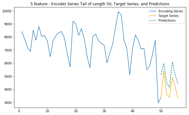
# Predict and plot

predict_and_plot_multi_f(encoder_input_data, decoder_target_data, 5060, mean_list=mean_list, model=model, dim=dim)
Main function - 5 features
This function uses internet, calls and sms traffic, as well as spatial (polar) coordinates to predict future internet traffic
def main_5(cell_id):
    global mean_list

    dim = 5 # nr. of features to use in the dataframe


    # Main 3 feature model
    model_to_use = '../01_Data/03_AWS outputs/model_5f_20181204_1142' # + timestr
    model = import_model(model_to_use)

    # Import model
    df_cdrs = import_source_data('../01_Data/03_AWS outputs/group_merged.csv')
    df_cdrs = add_spatial(df_cdrs)

    # Format and import data
    mean_list=[]
    df_cdrs, mean_list = scaler(df_cdrs, dim)
    keras_matrix = np.load("../02_Notebooks/keras_matrix_featurenr_5.dat")
    #keras_matrix = create_keras_matrix(df_cdrs,dim)

    y, y_list = df_cdrs.day.nunique(), df_cdrs.day.unique()
    d_dates_index = dict(zip(y_list,range(y)))

    # Generate encoder and decoder dataset
    encoder_input_data = (keras_matrix
                          [:, # all cell-towers
                          d_dates_index[val_enc_start.strftime('%Y-%m-%d')]: # start of training period
                           d_dates_index[val_enc_end.strftime('%Y-%m-%d')]+1, # end of training period
                          :] # all features
                         )

    # data from train_pred_start to train_pred_end
    decoder_target_data = (keras_matrix
                          [:, # all cell-towers
                          d_dates_index[val_pred_start.strftime('%Y-%m-%d')]: # start of pred period
                           d_dates_index[val_pred_end.strftime('%Y-%m-%d')]+1, # end of pred period
                          :] # all features to be used as target
                         )

    # Predict and plot
    predict_and_plot_multi_f(encoder_input_data, decoder_target_data, cell_id, mean_list=mean_list, model=model, dim=dim)
11. Reformatted spatial model
Using internet as the only non-spatial feature and using K-Means clustering to extract more consize spatial information from the coordinates
df_cdrs = import_source_data('../01_Data/03_AWS outputs/group_merged.csv')
df_cdrs = add_spatial(df_cdrs,polar=False)
del df_cdrs['calls']
del df_cdrs['sms']
df_cdrs.head()| day | CellID | internet | Lon | Lat | |
|---|---|---|---|---|---|
| 0 | 2013-10-31 | 1 | 57.799009 | 9.011491 | 45.358801 |
| 1 | 2013-10-31 | 2 | 57.914858 | 9.014491 | 45.358801 |
| 2 | 2013-10-31 | 3 | 58.038173 | 9.017492 | 45.358801 |
| 3 | 2013-10-31 | 4 | 57.463453 | 9.020492 | 45.358800 |
| 4 | 2013-10-31 | 5 | 52.171423 | 9.023493 | 45.358799 |
from scipy.cluster.vq import kmeans,vq
from scipy.spatial.distance import cdist

##### cluster data into K=1..10 clusters #####
#K, KM, centroids,D_k,cIdx,dist,avgWithinSS = kmeans.run_kmeans(X,10)

K = range(1,10)
X = df_cdrs[['Lon','Lat']].values

  # scipy.cluster.vq.kmeans
KM = [kmeans(X,k) for k in K] # apply kmeans 1 to 10
centroids = [cent for (cent,var) in KM]   # cluster centroids

D_k = [cdist(X, cent, 'euclidean') for cent in centroids]

cIdx = [np.argmin(D,axis=1) for D in D_k]
dist = [np.min(D,axis=1) for D in D_k]
avgWithinSS = [sum(d)/X.shape[0] for d in dist]
kIdx = 6
# plot elbow curve
fig = plt.figure()
ax = fig.add_subplot(111)
ax.plot(K, avgWithinSS, 'b*-')
ax.plot(K[kIdx], avgWithinSS[kIdx], marker='o', markersize=12,
markeredgewidth=2, markeredgecolor='r', markerfacecolor='None')
plt.grid(True)
plt.xlabel('Number of clusters')
plt.ylabel('Average within-cluster sum of squares')
tt = plt.title('Elbow for K-Means clustering') 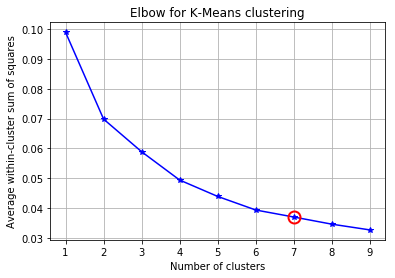
from sklearn.cluster import KMeans
km = KMeans(kIdx, init='k-means++') # initialize
km.fit(X)
c = km.predict(X) # classify into three clusterscarray([2, 2, 2, ..., 1, 1, 1], dtype=int32)
km.cluster_centers_array([[ 9.15837568, 45.41039273],
[ 9.26125249, 45.51608858],
[ 9.05955248, 45.4106078 ],
[ 9.06116834, 45.51637073],
[ 9.16225903, 45.51616683],
[ 9.25926288, 45.41032886]])
df_cdrs['Zone'] = c
del df_cdrs['Lon']
del df_cdrs['Lat']
df_cdrs.head()| day | CellID | internet | internet_scaled | Zone | |
|---|---|---|---|---|---|
| 0 | 2013-10-31 | 1 | 57.799009 | -0.477102 | 2 |
| 1 | 2013-10-31 | 2 | 57.914858 | -0.479278 | 2 |
| 2 | 2013-10-31 | 3 | 58.038173 | -0.481585 | 2 |
| 3 | 2013-10-31 | 4 | 57.463453 | -0.470914 | 2 |
| 4 | 2013-10-31 | 5 | 52.171423 | -0.468362 | 2 |
dim = 2
mean_list=[]
df_cdrs, mean_list = scaler(df_cdrs, dim)
keras_matrix = create_keras_matrix(df_cdrs,dim)
# Extracting training data
y, y_list = df_cdrs.day.nunique(), df_cdrs.day.unique()
d_dates_index = dict(zip(y_list,range(y)))
encoder_input_data = (keras_matrix
[:, # all cell-towers
d_dates_index[train_enc_start.strftime('%Y-%m-%d')]: # start of training period
d_dates_index[train_enc_end.strftime('%Y-%m-%d')]+1, # end of training period
:] # all features
)
# data from train_pred_start to train_pred_end
decoder_target_data = (keras_matrix
[:, # all cell-towers
d_dates_index[train_pred_start.strftime('%Y-%m-%d')]: # start of pred period
d_dates_index[train_pred_end.strftime('%Y-%m-%d')]+1, # end of pred period
:] # all features to be used as target
)
# we append a lagged history of the target series to the input data,
# so that we can train with teacher forcing
lagged_target_history = decoder_target_data[:,:-1,:]
encoder_input_data = np.concatenate([encoder_input_data, lagged_target_history], axis=1)# Building wavenet model for 5 feature prediction
from keras.models import Model
from keras.layers import Input, Conv1D, Dense, Dropout, Lambda, concatenate
from keras.optimizers import Adam
from keras.callbacks import EarlyStopping
# convolutional layer parameters
n_filters = 32
filter_width = 2
dilation_rates = [2**i for i in range(8)]
# define an input history series and pass it through a stack of dilated causal convolutions.
history_seq = Input(shape=(None, dim))
x = history_seq
for dilation_rate in dilation_rates:
x = Conv1D(filters=n_filters,
kernel_size=filter_width,
padding='causal',
dilation_rate=dilation_rate)(x)
x = Dense(128, activation='relu')(x)
x = Dropout(.2)(x)
x = Dense(dim)(x)
# extract the last 7 time steps as the training target
def slice(x, seq_length):
return x[:,-seq_length:,:]
pred_seq_train = Lambda(slice, arguments={'seq_length':pred_steps})(x)
model = Model(history_seq, pred_seq_train)
model.summary()
# Fit the model on the training data
batch_size = 2**11
epochs = 100
model.compile(Adam(), loss='mean_absolute_error')
monitor = EarlyStopping(monitor='val_loss', min_delta=1e-3, patience=5, verbose=1, mode='auto')
history = model.fit(encoder_input_data, decoder_target_data,
batch_size=batch_size,
callbacks=[monitor],
epochs=epochs,
validation_split=0.2)_________________________________________________________________
Layer (type) Output Shape Param #
=================================================================
input_2 (InputLayer) (None, None, 2) 0
_________________________________________________________________
conv1d_9 (Conv1D) (None, None, 32) 160
_________________________________________________________________
conv1d_10 (Conv1D) (None, None, 32) 2080
_________________________________________________________________
conv1d_11 (Conv1D) (None, None, 32) 2080
_________________________________________________________________
conv1d_12 (Conv1D) (None, None, 32) 2080
_________________________________________________________________
conv1d_13 (Conv1D) (None, None, 32) 2080
_________________________________________________________________
conv1d_14 (Conv1D) (None, None, 32) 2080
_________________________________________________________________
conv1d_15 (Conv1D) (None, None, 32) 2080
_________________________________________________________________
conv1d_16 (Conv1D) (None, None, 32) 2080
_________________________________________________________________
dense_3 (Dense) (None, None, 128) 4224
_________________________________________________________________
dropout_2 (Dropout) (None, None, 128) 0
_________________________________________________________________
dense_4 (Dense) (None, None, 2) 258
_________________________________________________________________
lambda_2 (Lambda) (None, None, 2) 0
=================================================================
Total params: 19,202
Trainable params: 19,202
Non-trainable params: 0
_________________________________________________________________
Train on 8000 samples, validate on 2000 samples
Epoch 1/100
8000/8000 [==============================] - 16s 2ms/step - loss: 0.1256 - val_loss: 0.0687
Epoch 2/100
8000/8000 [==============================] - 11s 1ms/step - loss: 0.1076 - val_loss: 0.0709
Epoch 3/100
8000/8000 [==============================] - 10s 1ms/step - loss: 0.0965 - val_loss: 0.0577
Epoch 4/100
8000/8000 [==============================] - 10s 1ms/step - loss: 0.0854 - val_loss: 0.0524
Epoch 5/100
8000/8000 [==============================] - 10s 1ms/step - loss: 0.0787 - val_loss: 0.0560
Epoch 6/100
8000/8000 [==============================] - 10s 1ms/step - loss: 0.0755 - val_loss: 0.0517
Epoch 7/100
8000/8000 [==============================] - 11s 1ms/step - loss: 0.0725 - val_loss: 0.0511
Epoch 8/100
8000/8000 [==============================] - 9s 1ms/step - loss: 0.0707 - val_loss: 0.0498
Epoch 9/100
8000/8000 [==============================] - 9s 1ms/step - loss: 0.0686 - val_loss: 0.0499
Epoch 10/100
8000/8000 [==============================] - 9s 1ms/step - loss: 0.0674 - val_loss: 0.0486
Epoch 11/100
8000/8000 [==============================] - 10s 1ms/step - loss: 0.0665 - val_loss: 0.0485
Epoch 12/100
8000/8000 [==============================] - 9s 1ms/step - loss: 0.0658 - val_loss: 0.0491
Epoch 13/100
8000/8000 [==============================] - 9s 1ms/step - loss: 0.0650 - val_loss: 0.0485
Epoch 14/100
8000/8000 [==============================] - 9s 1ms/step - loss: 0.0646 - val_loss: 0.0480
Epoch 15/100
8000/8000 [==============================] - 9s 1ms/step - loss: 0.0642 - val_loss: 0.0482
Epoch 00015: early stopping
model_name='../01_Data/03_AWS outputs/model_3f_internet_zoned_20181205_1135'

# serialize model to JSON
model_json = model.to_json()
with open(model_name+".json", "w") as json_file:
    json_file.write(model_json)
# serialize weights to HDF5
model.save_weights(model_name+".h5")
print(f"Saved {model_name} to disk")
Saved ../01_Data/03_AWS outputs/model_3f_internet_zoned_20181205_1135 to disk
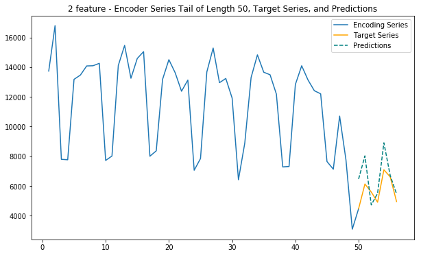
Main function - 2 feature (internet & location cluster)
This function uses internet traffic and cell location information (as 7 clusters) to predict future internet traffic
def main_2_internet_zoned(cell_id):
    global mean_list

    dim = 2 # nr. of features to use in the dataframe


    # Main 3 feature model
    model_to_use = '../01_Data/03_AWS outputs/model_3f_internet_zoned_20181205_1135'
    model = import_model(model_to_use)

    # Import model
    df_cdrs = import_source_data('../01_Data/03_AWS outputs/group_merged.csv')
    df_cdrs = add_spatial(df_cdrs)

    # Format and import data
    mean_list=[]
    df_cdrs, mean_list = scaler(df_cdrs, dim)
    keras_matrix = np.load("../02_Notebooks/keras_matrix_internet+zones_featurenr_2.dat")
    #keras_matrix = create_keras_matrix(df_cdrs,dim)

    y, y_list = df_cdrs.day.nunique(), df_cdrs.day.unique()
    d_dates_index = dict(zip(y_list,range(y)))

    # Generate encoder and decoder dataset
    encoder_input_data = (keras_matrix
                          [:, # all cell-towers
                          d_dates_index[val_enc_start.strftime('%Y-%m-%d')]: # start of training period
                           d_dates_index[val_enc_end.strftime('%Y-%m-%d')]+1, # end of training period
                          :] # all features
                         )

    # data from train_pred_start to train_pred_end
    decoder_target_data = (keras_matrix
                          [:, # all cell-towers
                          d_dates_index[val_pred_start.strftime('%Y-%m-%d')]: # start of pred period
                           d_dates_index[val_pred_end.strftime('%Y-%m-%d')]+1, # end of pred period
                          :] # all features to be used as target
                         )

    # Predict and plot
    predict_and_plot_multi_f(encoder_input_data, decoder_target_data, cell_id, mean_list=mean_list, model=model, dim=dim)
12. Results for selected regions
Below some results are to be found from key areas in Milan, showing the performance of the various models
# Main square: 6169

cell_id = 6169

main_1(cell_id)
main_3(cell_id)
main_5(cell_id)
main_2_internet_zoned(cell_id)
Loaded ../01_Data/03_AWS outputs/model_1f from disk
Loaded ../01_Data/03_AWS outputs/model_3f_20181203_1651 from disk
Loaded ../01_Data/03_AWS outputs/model_5f_20181204_1142 from disk
Loaded ../01_Data/03_AWS outputs/model_3f_internet_zoned_20181205_1135 from disk

# Train station: 6064

cell_id = 6064

main_1(cell_id)
main_3(cell_id)
main_5(cell_id)
main_2_internet_zoned(cell_id)
Loaded ../01_Data/03_AWS outputs/model_1f from disk
Loaded ../01_Data/03_AWS outputs/model_3f_20181203_1651 from disk
Loaded ../01_Data/03_AWS outputs/model_5f_20181204_1142 from disk
Loaded ../01_Data/03_AWS outputs/model_3f_internet_zoned_20181205_1135 from disk

# Duomo: 5060

cell_id = 5060

main_1(cell_id)
main_3(cell_id)
main_5(cell_id)
main_2_internet_zoned(cell_id)
Loaded ../01_Data/03_AWS outputs/model_1f from disk
Loaded ../01_Data/03_AWS outputs/model_3f_20181203_1651 from disk
Loaded ../01_Data/03_AWS outputs/model_5f_20181204_1142 from disk
Loaded ../01_Data/03_AWS outputs/model_3f_internet_zoned_20181205_1135 from disk


13. Extracting predictions for dashboard creation
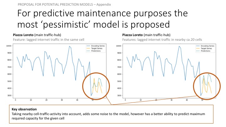
Preaparing the data using the 5-dimensional model. Using the 5-dimensional model for dashboard building, as that is the most pessimistic about cell-traffic growth.
global mean_list

dim = 5 # nr. of features to use in the dataframe


# Main 3 feature model
model_to_use = '../01_Data/03_AWS outputs/model_5f_20181204_1142' # + timestr
model = import_model(model_to_use)

# Import model
df_cdrs = import_source_data('../01_Data/03_AWS outputs/group_merged.csv')
df_cdrs = add_spatial(df_cdrs)

# Format and import data
mean_list=[]
df_cdrs, mean_list = scaler(df_cdrs, dim)
keras_matrix = np.load("../02_Notebooks/keras_matrix_featurenr_5.dat")
#keras_matrix = create_keras_matrix(df_cdrs,dim)

y, y_list = df_cdrs.day.nunique(), df_cdrs.day.unique()
d_dates_index = dict(zip(y_list,range(y)))

# Generate encoder and decoder dataset
encoder_input_data = (keras_matrix
                      [:, # all cell-towers
                      d_dates_index[val_enc_start.strftime('%Y-%m-%d')]: # start of training period
                       d_dates_index[val_enc_end.strftime('%Y-%m-%d')]+1, # end of training period
                      :] # all features
                     )

# data from train_pred_start to train_pred_end
decoder_target_data = (keras_matrix
                      [:, # all cell-towers
                      d_dates_index[val_pred_start.strftime('%Y-%m-%d')]: # start of pred period
                       d_dates_index[val_pred_end.strftime('%Y-%m-%d')]+1, # end of pred period
                      :] # all features to be used as target
                     )
Loaded ../01_Data/03_AWS outputs/model_5f_20181204_1142 from disk
encoder_input_data.shape(10000, 49, 5)
Extraction
Extracting 7-day prediction sequences for each of the 10000 cell towers
14. Alarm system
Creating an alarm system that indicates which cell-towers have at least 60% + / - traffic change in the next 7-days vs. the mean of the last 40-days
from IPython.display import clear_output
pred_sequence = np.zeros((encoder_input_data.shape[0],pred_steps,dim)) # initialize output (pred_steps time steps)

for cell_ID in range(encoder_input_data.shape[0]):
    clear_output()
    print(cell_ID)

    history_seq = encoder_input_data[cell_ID:cell_ID+1,:,:]

    for i in range(pred_steps): #pred_steps=7 at beginning of code

        last_step_pred=model.predict(history_seq)[0,-1,:]
        pred_sequence[cell_ID,i,:] = last_step_pred

        # add the next time step prediction to the history sequence
        history_seq = np.concatenate([history_seq,
                                           last_step_pred.reshape(-1,1,dim)], axis=1)

print(f'Pred sequence prepared for all towers. Final shape {pred_sequence.shape}')
pred_sequence.dump("pred_sequence_20181204_1451.dat")
pred_sequence = np.load("pred_sequence_20181204_1451.dat")# Scaling data back to real world units
for i in range(10000):
encoder_input_data[i,:,:] = np.expm1(encoder_input_data[i,:,:] + mean_list[i])
pred_sequence[i,:,:] = np.expm1(pred_sequence[i,:,:] + mean_list[i])# Extracing internet traffic of last 40 days for each tower, and taking the mean
last_forty_mean = np.mean(encoder_input_data[:,-40:,0],axis=1)
last_forty_mean = np.where(last_forty_mean==0,0.1,last_forty_mean) # substituting 0-s with 0.1 to enable calcs
last_forty_mean.shape(10000,)
# Extracting the expected internet traffic for the next 7 days for each tower and taking
next_seven_max = np.max(pred_sequence[:,:,0],axis=1)
next_seven_min = np.min(pred_sequence[:,:,0],axis=1)
print(next_seven_max.shape)
(10000,)
# Calculating % diff between mean of last 7 days and next 7 days min and max
growth = ((next_seven_max-last_forty_mean)/last_forty_mean)*100
shrinkage = ((next_seven_min-last_forty_mean)/last_forty_mean)*100
threshold = 60 #%import plotly.plotly as py
import plotly.graph_objs as go
x = np.where(growth>threshold)[0]+1
y = growth[growth>threshold]
# Create a trace
trace = go.Bar(
x = x,
y = y
)
data = [trace]
py.iplot(data, filename='basic-line')High five! You successfully sent some data to your account on plotly. View your plot in your browser at https://plot.ly/~krisz.sandor/0 or inside your plot.ly account where it is named 'basic-line'
high_growth = list(zip(np.where(growth>threshold)[0]+1,growth[growth>threshold]))

print(f'Cell towers with at least {threshold}% expected traffic growth: {high_growth}')
#plt.plot(np.where(growth>threshold)[0],growth[growth>threshold])
Cell towers with at least 60% expected traffic growth: [(814, 66.93866006968008), (3936, 75.09995857223389), (4136, 77.55330815818837), (4140, 64.96232330482368), (4141, 74.97279829033853), (4236, 75.94500582181918), (4241, 63.91302465738832), (4632, 70.50906919857434), (4633, 62.16145895137404), (4634, 62.60213430436957), (4731, 64.50277580034849), (4732, 70.9975885227163), (4733, 73.08078206974949), (4734, 71.29920549828279), (4831, 62.05815315326537), (4832, 69.1531248886856), (4833, 71.85924136173747), (4834, 75.40826283157858), (4835, 66.65852371175299), (4837, 60.85333476959609), (4934, 61.42642754609903), (4940, 62.007212990375194), (5039, 64.39630989378534), (5139, 79.21231098746337), (5238, 77.42990560987654), (5816, 68.3516251981003), (5916, 77.95917011476064), (5917, 76.95966391787435), (6172, 77.17692067917409), (7178, 73.13060803775497), (7277, 66.99386455440506), (7278, 78.8551969081368), (7279, 99.3974583047096), (7280, 78.04388192505137), (7377, 65.79338939936086), (7378, 66.35046709286505), (7379, 79.07796926434906), (7479, 66.95840250047291), (7776, 60.68202702116308), (7777, 75.49973254483936), (7778, 80.92741775556323)]
alarm_df = pd.DataFrame([range(1,10001),np.where(growth>threshold,1,0),np.where(shrinkage<-threshold,1,0)]).T
alarm_df.columns = ['CellID','Growth_Alarm','Shrinkage_A']
alarm_df.to_csv('alarm_df_for_tableau.csv')
For a detailed visual alarm system dashboard example, visit: https://public.tableau.com/profile/krisztian.sandor#!/vizhome/Kojak_v1_1/Internet2